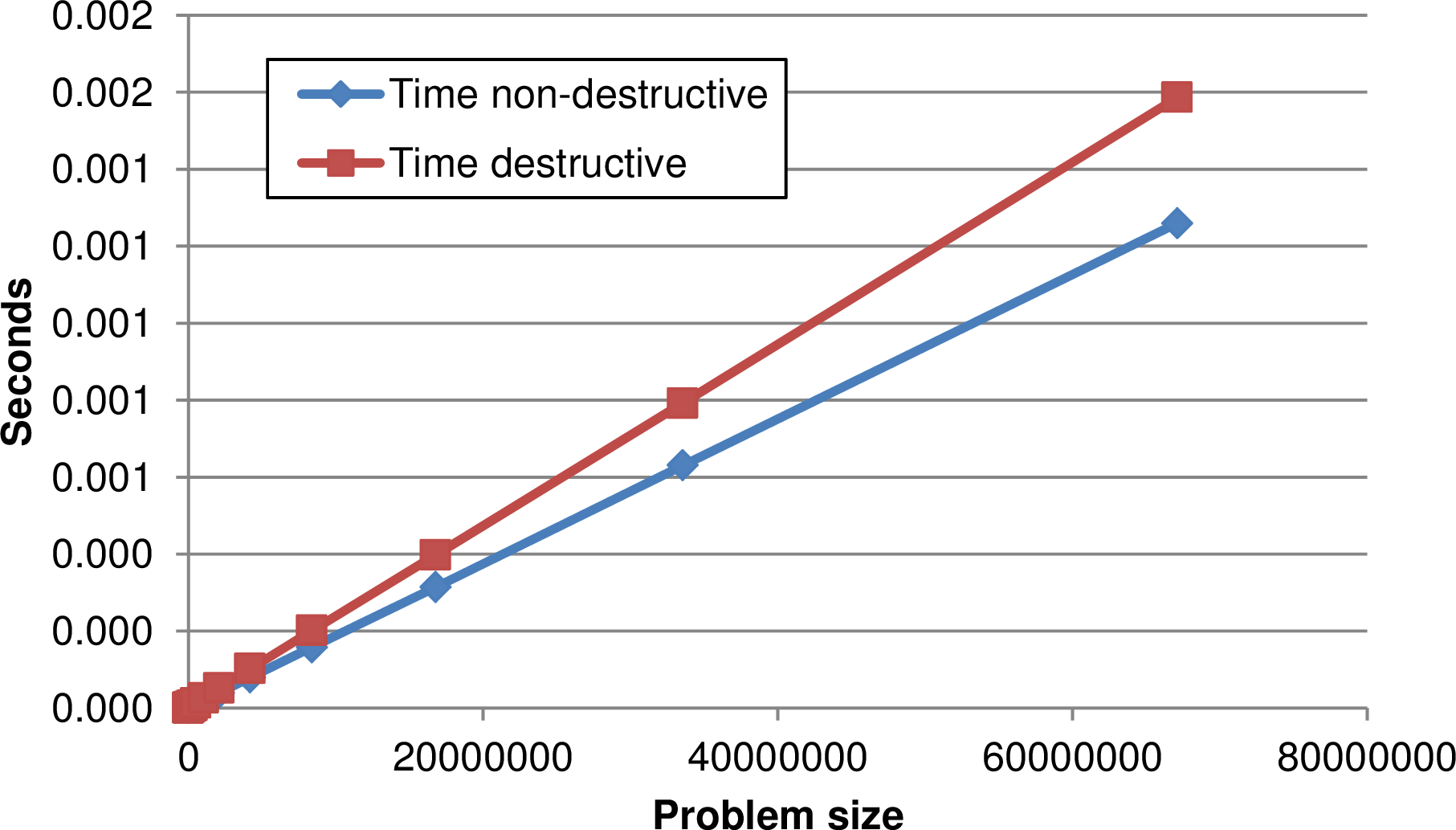
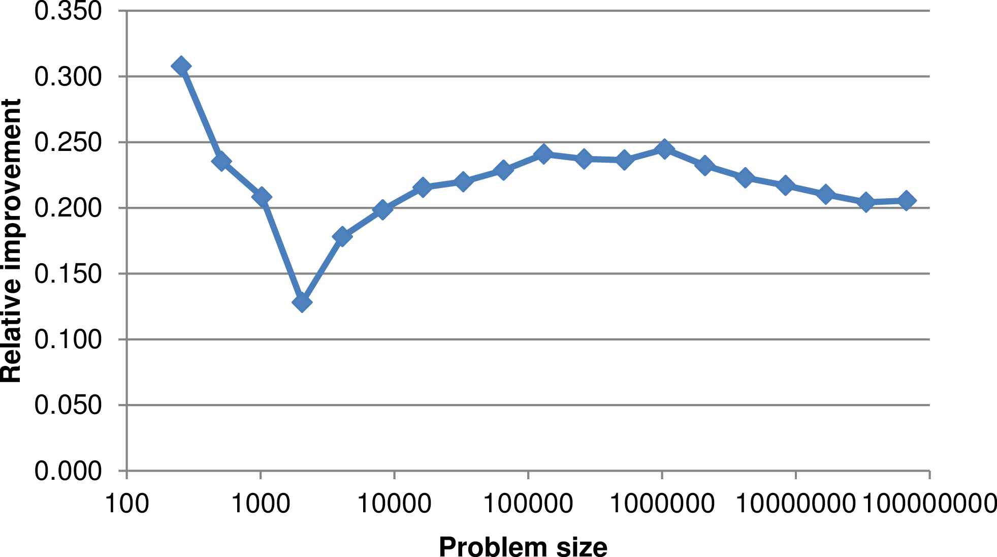
Figure 4.7: Benchmark for non-destructive streams vs. destructive streams with different
stream sizes showing robust improvement for larger problem sizes with non-destructive streams.
We continue with a concrete description on how we execute a stack- and stream-based simulation on a static grid. Due to the static grid, we assume the grid structure already stored in the structure stream.
In order to run a simulation for solving the hyperbolic equations with our stack-based communication system, we continue determining further buffer requirements. We introduce different stack types:
Then, the basic stack for grid storage, usable for a pure grid traversal without any computations, is
given by
| Stack S | Description of purpose | Classification |
| Sfbstructure | Grid representation | persistent |
Depending on the simulation requirements, additional stacks are used. For a simulation with a DG method on a static grid and flux computations requiring an edge-based communication, this leads to the following additional stacks:
| Stack S | Description of purpose | Classification |
| SfbsimCellData | Storage for cell data (e.g. DoF) | persistent |
| SlrsimEdgeComm | Edge data communicated to adjacent cells | semi-persistent |
| StsimEdgeBuffer | Buffer for data exchange via edges | semi-persistent |
The buffer StsimEdgeBuffer is required to buffer the communication data during the forward traversal. This data from adjacent cells is then fetched during the backward traversal.
With our knowledge on the basics of a hyperbolic simulation, we are going to assemble a simulation with the stack- and stream-based approach introduced in the previous Sections.
For flux computations, we do not follow the approach of splitting the flux computations as suggested in [BBSV10] which basically avoids computing the flux based on the DoF on each cell’s edge. Such an approach is not applicable with the Rusanov flux solvers from Section 2.10 as well as many other solvers.
A single time step is then computed with the following algorithmic pattern using a forward and backward traversal.
Additionally to the flux parameters, the inner cell radius is also transfered for computing the CFL condition (see Section 2.13) to allow a time step size computation which depends on the inner cell radius of each cell.
Flux updates for edges of type old have previously been pushed to the corresponding left or right edge communication stack and are read from the respective stack.
An alternative approach for flux computations presented in the traversal-intermediate processing is computing the flux updates during the first forward traversal before pushing the flux parameters to the edge buffer (see [SBB12] for an implementation). This avoids the mid-processing and, thus, also additional bandwidth requirements; However, it does not yield the optimization of vectorized flux evaluation for finite volume simulations (see Section 4.10.4) and hence was not considered in this work.
With a software concept using input- and output-streams and temporary stacks only (cf. [MRB12,Nec09,Wei09]), all the data has to be read from one memory location and written to another memory location. Among others, this results in increased cache utilization due to additional memory being accessed and additional cache blocks used. Another performance aspect are additional index computations for the second stack.
We tested this hypothesis with two different benchmarks based on an array of size n. Both benchmarks operate on an array of integers and successively increment the stored values. The first benchmark operates in-situ, reading a floating point value, incrementing it and writing the data back to the same array entry, whereas the second benchmark writes the result to an additional array.
Figure 4.7 shows results for both benchmarks with different block sizes. It suggests that non-destructive streams are mandatory for memory performance. This leads to a robust performance improvement of more than 20% for larger streams using non-destructive streams.
Thus, we use an approach with non-destructive access to our stack structures and further motivate this by highlighting possible applications in our algorithm:
This yields two different kinds of non-destructive streams. Assuming e.g. a grid traversal in forward direction accessing cell data, a top-down stream is used to iterate over the stack data top-down. A bottom-up stream can be used in a similar way to start iterating over the data from the very first element on the bottom of the stack. All these stream operations do not remove or add any data to stack, they only update the stack entries.
Optimizing our input/output scheme with these non-destructive streams, this modifies our stack system used for the simulation on static grids (Sec. 4.5.2) in the following way:
Forward traversal:
Backward traversal:
We just presented the modifications of our stack system to a non-destructive system with a static grid. Next, we continue with the adaptivity traversals.