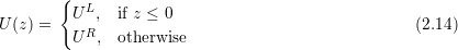
With the evaluation of the flux function only involving pairs of selected conserved quantities on the edge from the local and adjacent triangle, we can interpret this as a Riemann problem, for which we consider two different ways of handling it:
Since both types of Riemann solvers can be implemented with the same interfaces, we only introduce the most frequently used flux solver for higher-order methods: the local Lax-Friedrichs flux, also called Rusanov flux.
We consider flux computations which are based on the one-dimensional representation in edge space (see Section 2.9) and a constant state representation of the solution on each side of the edge with UiL and UiR. This leads to a Riemann problem in edge space with
with the function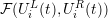 (UiL(t),UiR(t)) and F(U) with evaluating a Riemann problem on an edge
whereas F evaluates the flux function inside the reference triangle.
(UiL(t),UiR(t)) and F(U) with evaluating a Riemann problem on an edge
whereas F evaluates the flux function inside the reference triangle.
Averaging both points by using the equation
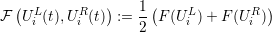 | (2.15) |
and using this average value as the flux over the edges would result in a numerically unstable simulation. Therefore, an artificial numerical damping is frequently introduced to overcome these instabilities. This damping is often referred to as numerical diffusion or artificial viscosity [LeV02].
One example of such fluxes involving a numerical diffusion is the Rusanov flux [Rus62]. This flux function introduces a diffusive term with its magnitude depending on the speed of the information propagation. This propagation speed is given by the eigenvalues of the Jacobian matrix of the flux (see Section 1.2.1 and Section 1.2.2 for concrete examples). For the two-dimensional Lax-Friedrichs flux function for Riemann problems given by UjL, UjR and F(U) we use the flux function [BGN00]
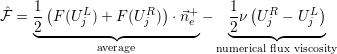 | (2.16) |
with the numerical Lax-Friedrichs viscosity component given by
 | (2.17) |
Here, JF (U) is the Jacobian of the function F with respect to the conserved quantities U.
With higher-order spatial discretization methods, artificial oscillations can be generated in the solution. To avoid these oscillations, limiters can be used to modify the solution based on data either adjacent via edges or vertices (see [GW08,HW08]). Since the interfaces for edge-based data exchange required for flux computations and vertex-based exchange for visualization as further explained in Sec. 4.3.4 are considered in the framework, we resigned implementing limiters.
An alternative approach to avoid oscillations is to introduce additional artificial viscosity which was already applied to DG simulations for atmospheric simulations in [Mül12]. Since this part of the thesis focuses on framework requirements for simulations with higher-order DG, we used a similar concept to avoid implementation of challenging flux limiters. For DG simulations and polynomial degrees which are larger than 2, we slightly slow down the fluid’s velocity while still being able to test our algorithms for running higher-order simulations on dynamically adaptive grids.