These html pages are based on the
PhD thesis "Cluster-Based Parallelization of Simulations on Dynamically Adaptive Grids and Dynamic Resource Management" by Martin Schreiber.
There is also
more information and a PDF version available.
1.2 Examples of hyperbolic systems
Up to now, the governing equation was derived using the conserved quantities U, the flux function F
and the source term S. This section concretizes these terms by presenting two different scenarios:
simulations assuming a shallow water, based on the shallow water equations, and compressible gas
simulations neglecting the viscosity, based on the Euler equations.
1.2.1 Shallow water equations
Simulation of water with free surfaces is mainly considered to be a three-dimensional problem. Using
depth averaged Navier-Stokes equations (see e.g. [Tor01]), this three-dimensional problem can be
reformulated to a two-dimensional problem under special assumptions. Among others, vertical moving
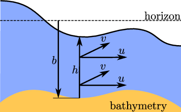
fluid is assumed to be negligible. This leads to the so-called shallow water equations (SWE) giving a
description of the water by its water surface height h, the two-dimensional velocity components (u,v)T
and the bathymetry b.
Several ways of a mathematical representation of these quantities are used such as specifying the
water surface relative to the horizon or to the bathymetry. We use the shallow water formulation
storing the bathymetry b relative to the steady state of the water and the water surface height h
relative to the bathymetry [LeV02,BSA12]. For a sea without waves and tidals, b is positive for terrain
and negative for the sea floor.
By using the velocity components as conserved quantities, this is considered not to be a
momentum conserving formulation. Thus, instead of storing the velocity components, we store both
momentums hu and hv as the conserved quantities. This leads to the tuple of conserved
quantities
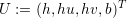 for
each nodal point with a sketch in Fig. 1.2. Despite that hu and hv are frequently described as
momentum, we should be aware that h actually describes the height of a volume above a unit area.
Therefore, this momentum may not be seen as a momentum per cell, but rather as momentum per
unit area.
for
each nodal point with a sketch in Fig. 1.2. Despite that hu and hv are frequently described as
momentum, we should be aware that h actually describes the height of a volume above a unit area.
Therefore, this momentum may not be seen as a momentum per cell, but rather as momentum per
unit area.
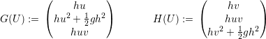
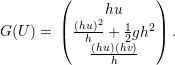
Using this form based on the conserved quantities and assuming a constant bathymetry without
loss of generality, we formulate the flux functions G and H (see Eq. (1.4)):
For the flux computations (see Section 2.10), we need the eigenvalues of the Jacobian  . We
start by substituting all v with
. We
start by substituting all v with  and u with
  . This yields
 | (1.6) |
By computing the derivative with respect to each of the conserved quantities (h,hu), this
yields
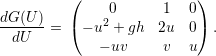 | (1.7) |
Finally, the sorted eigenvalues of the Jacobian of G are given by
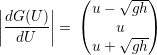 | (1.8) |
which are required for the computation of the maximum time step size.
1.2.2 Euler equations
For compressible flow with a negligible viscosity, the Navier-Stokes equations can be simplified to the
so-called Euler equations which belongs to one of the standard models used for fluid simulations. For
this work, we consider the two-dimensional Euler equations with the conserved quantities given by
U := (ρ,ρu,ρv,E) with ρ being the fluid density, (u,v)T the velocity components and E the
energy. The similarities to the shallow water equations are clearly visible by considering the
density instead of the height of a water surface. The flux terms G and H are then given
with
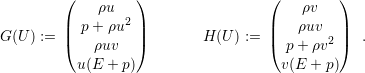 | (1.9) |
In this terms, the pressure p depends on the type of gas being simulated. For our simulations, we only
consider an isothermal gas with
 and
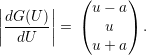
a constant a specific to the simulated gas (see [LeV02], page 298). For the computation of the wave
speed, the Jacobian G is given by
and
a constant a specific to the simulated gas (see [LeV02], page 298). For the computation of the wave
speed, the Jacobian G is given by
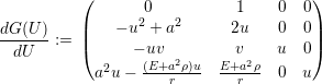 with
the associated eigenvalues of its Jacobian
with
the associated eigenvalues of its Jacobian
 | (1.10) |