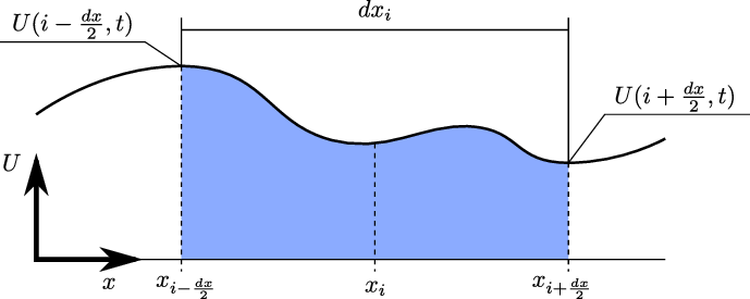
Figure 1.1: Conservation of quantities in an infinitesimal small one-dimensional shallow water
simulation interval.
As a starting point for the derivation of the continuity equation, we consider a one-dimensional simulation scenario (see Fig. 1.1) placed at an infinitesimal small interval of size dx. The quantities we are interested in are given continuously by Û(x,t) ∈ ℝn for n conserved quantities at position x at time t. Furthermore a so-called flux function F(Û(x,t)) : ℝn → ℝn is given. Its values account for the change of the conserved quantities at a particular position x ∈ ℝ for the current state Û(x,t) at time t ∈ ℝ. To give an example, we consider a single simulated quantity, such as the gas density or the water height, only. Based upon an advection model assuming a constant advection speed vc of conserved quantity, then, the flux function is given by F(Û(x,t)) := vc Û(x,t).
A sketch of a single interval I(i) := [xi - ;xi +
;xi +  ] of our model is given in Figure 1.1. In each
interval, we consider the average quantities Û(i)(t) :=
] of our model is given in Figure 1.1. In each
interval, we consider the average quantities Û(i)(t) :=  ∫
I(i)Û(x,t)dx. We further should track the
incoming and outgoing quantities at the interval boundaries dI(i) := {xi -
∫
I(i)Û(x,t)dx. We further should track the
incoming and outgoing quantities at the interval boundaries dI(i) := {xi - ,xi +
,xi +  } with the change
of quantities given by the flux function which is evaluated at the corresponding boundary points.
Assuming a change in conserved quantities Û(i) in an interval with a mesh size dx in space and
time-step size dt, we describe the change of the system by the change on the boundaries and
get
} with the change
of quantities given by the flux function which is evaluated at the corresponding boundary points.
Assuming a change in conserved quantities Û(i) in an interval with a mesh size dx in space and
time-step size dt, we describe the change of the system by the change on the boundaries and
get
 | (1.1) |
The left side of Equation (1.1) represents the average of conserved quantities in the interval I(i)) at the next time step whereas the right side represents the old state and the change of this state over time via the flux at both interval boundaries.
These terms can be rearranged to a forward finite differencing scheme, yielding
 | (1.2) |
Assuming that the solution Û is sufficiently smooth, the limits dt → 0 and dx → 0 of (1.2) then gives the one-dimensional continuity equation
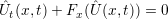 | (1.3) |
with Û as the set of conserved quantities and the subscript x and t used as an abbreviation for the derivative w.r.t. to space and time.
We further add a source term S(Û(x,t)) at the right side of the Eq. (1.3). This source term is frequently used to account for non-homogeneous effects such as external forces, changing bathymetry, etc. An extension to two and three dimensions is directly given by including flux functions with a derivative with respect to y and z. For flux functions based on two-dimensional conserved quantities such as the momentum, we use the notation G for the flux function derived to x and H derived to y
 | (1.4) |
Using the gradient ∇ = ( ,
, )T and F(Û,t) = G(Û,t)(1,0)T + H(Û,t)(0,1)T , this equation can be
written compactly with the two-dimensional equation of conservation
)T and F(Û,t) = G(Û,t)(1,0)T + H(Û,t)(0,1)T , this equation can be
written compactly with the two-dimensional equation of conservation
 | (1.5) |