These html pages are based on the PhD thesis "Cluster-Based Parallelization of Simulations on Dynamically Adaptive Grids and Dynamic Resource Management" by Martin Schreiber.
There is also more information and a PDF version available.

4.6 Adaptivity

We introduce two additional stack systems for adaptivity. The first one accounts for the current adaptivity state in each cell, the second one for the adaptivity communication information to create a conforming grid, a grid without hanging nodes, by inserting additional edges.


Stack or stream S

Comment


SlradaptiveEdgeComm

Left and right stack for edge communication information to transfer the three different adaptivity markers M
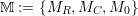


SadaptiveState

Adaptivity state for each cell, see Fig. 4.8


The stacks SlradaptiveEdgeComm are then used to forward three different adaptivity markers

M := {MR,  MC ,M0 }
to adjacent cells, requesting a refinement on an edge, a coarsening or no adaptivity request.

We store the adaptivity state on a separate stack SadaptiveState. This allows for the computation of the conforming transitions without touching the simulation cell data stack in the middle traversals to reduce memory bandwidth requirements during the adaptivity traversals.

The adaptivity process (for optimizations, see Sections 4.10.3 and 5.8.2) is then given with a three-pass system which we can execute iteratively:


pict

Figure 4.8: Different adaptivity states of each triangle. The red dashed lines represent the new edges of the refined triangle or the removed edges for a coarsening operation joining two triangles [SBB12].

1.
First forward traversal - marking of refine/coarsen operation requests:
Based on the adaptivity indicators (See Section 2.12.5), three adaptivity states are introduced: each cell either requests a (3) local refine operation on the cell, a (2) joining with another cell or (0) no adaptivity request, see Fig. 4.8. Adaptivity markers are then forwarded to adjacent cells similar to the middle traverals which are discussed next.
2.
Middle backward/forward traversals - determine conforming transition:
To create a conforming grid, a conforming transition of the grid cells to the new grid has to be determined. This requires two markers forwarding refinement and coarsening operations. The middle traversals are done by successively executing backward and forward traversals until a conforming grid state is reached. All edges then have to be marked with the same markers. Further details on the creation of this conforming transition are given in Section 4.6.3.
3.
Applying conforming transition to grid cell data:
The last backward traversal applies the transition states determined by refining/coarsening cells and the actual modification of the element data. Regarding the persistent cell data stored on the stack system, this is accomplished by streaming the cell data and inserting or removing additional cells. For interpolation and restriction operations, see Section 2.12.

4.6.1 Refinement

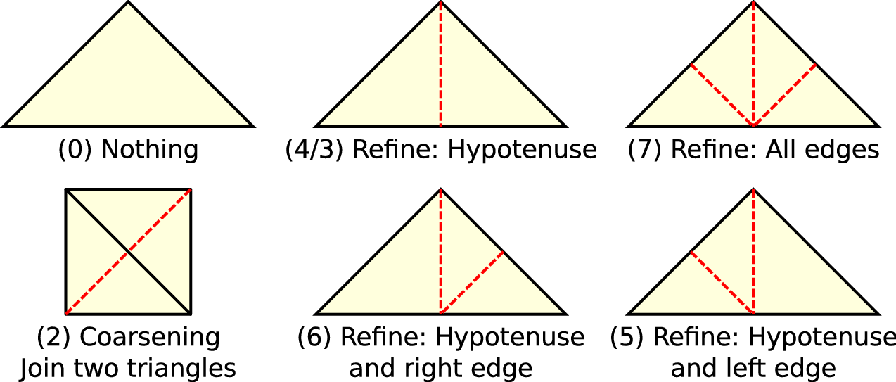
A single forward or backward traversal does not propagate information to all adjacent cells. This is due to edge communication information only propagated to cells which are traversed in the direction of the SFC.

Hence, additional forward and backward traversals are required. The determination of the conforming transition is thus similar to an iterative method: As many iterative smoother steps are done until the residual, in our case the conforming state, is reached.

Considering all possible refinement states required to create a conforming grid, additional split states for a refinement triggered via e3, e2 and via both edges are required (See Fig. 4.8 for refinement states (4) to (7)).


pict

Figure 4.9: Basic adaptive refinement traversals. Adaptivity with a forward and two backward traversals. Note, that the 1st backward traversal was only required to determine a conforming adaptive state.

4.6.2 Coarsening


pict

Figure 4.10: Coarsening agreement of cells due to adaptivity traversals. During the first forward traversal, coarsening markers are forwarded along the triangle legs of cells requesting a coarsening operation. A successful coarsening is applied with the last backward traversal  [SBB12].

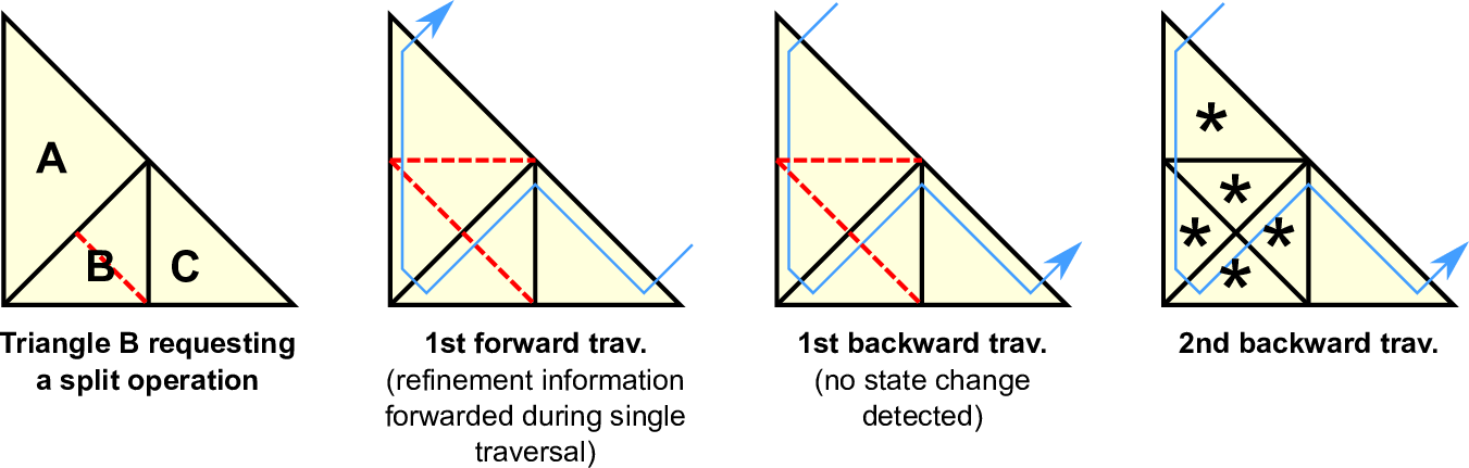
Using the knowledge on spacetrees and with the constraint of no hanging nodes, a coarsening operation is only permitted under particular circumstances. Figure 4.10 gives a sketch of a coarsening operation. Two constraints have to be fulfilled for a valid, conforming grid generating coarsening operation:

1.
The first constraint is obviously given by the spacetree with only leaf nodes with the same parent node allowed to coarsen. Following the recursive grammar from Section 4.1, these leaf nodes always share an edge with one of the triangle legs and different triangle legs (left or right) for the leaf nodes.
2.
The second constraint is raised by the conforming grid property: if only both leaf nodes are joined to a single cell, the resulting triangle can have a hanging node on its hypotenuse. This also demands for coarsening of both cells adjacent to the hypotenuse of the coarsened triangle.

The requirements driven by both constraints lead to a “diamond”-like shape [HDJ04] of triangles involved in coarsening as depicted in Fig. 4.10. Note, that the diamond is created by the touching triangle legs of the four triangles. In case of a coarsening request, a conforming grid can only be obtained if all four involved triangles agree to the coarsening and thus forward coarsening markers MC along all triangle leg edges. Using the cell traversal order induced by the Sierpiński SFC, a forward followed by a backward traversal is sufficient to propagate the coarsening information: during the first forward traversal, the coarsening request markers MC are propagated via the triangle legs to the adjacent cells accounting for the diamond like shape. As soon as one cell does not request a coarsening, the marker is not forwarded anymore. In case of the coarsening information not being fully propagated to the last cell in the diamond, the coarsening requests are all invalidated during the backward traversal by the same approach.

In case of a refinement marker forwarded via an edge to a cell that requests a coarsening, this coarsening becomes invalid and the state is transferred to one of the corresponding refinement states (3)-(7).

Hence, the computational grid can be a superset of the required mesh.

4.6.3 Termination of adaptivity traversals

One approach for testing for a transition state resulting in a conforming grid was suggested in [BBSV10]. With this approach, the traversal is stopped if no change of state is determined (cf. Fig. 4.9).

This number of conforming grid traversals is limited even with the cascade of edge insertions to avoid hanging nodes. We consider the two possible reasons for cascades.

(a)
A pseudo cascade forwards the information on the hanging node to the adjacent cell with both considered cells sharing only the hypotenuse. In this case, the forwarding of refinement markers directly leads to a conforming grid once the marker has been forwarded.
(b)
A real cascade forwards the refinement marker via the hypotenuse to a cell sharing one of its cathetus. This adjacent cell is related to a leaf node one level higher in the refinement tree. Thus, the cascading process can only occur on higher levels, directly leading to the upper limit given by the refinement depth. With the refinement markers forwarded at least once in each pair of forward and backward traversal, this assures the termination of the adaptivity algorithm.

Joining adaptivity and time step traversals

The adaptivity traversals can be combined with the simulation traversals. Since its feasibility was already shown in [Nec09,Wei09], this was not further considered in this work.