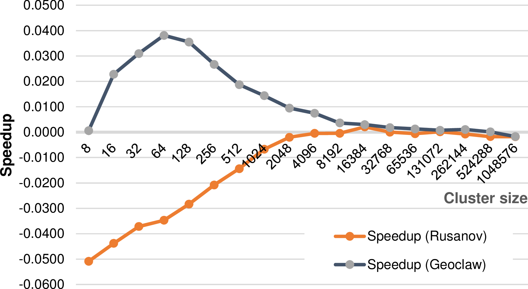
Figure 5.28: Performance speed up and speed down if avoiding duplicated reduction of
replicated data.
We continue with an overview of possible optimizations:
Using the replicated communication scheme (see Section 5.2), there are basically two ways to reduce the replicated data:
First, we have to make a decision which cluster should compute the reduction. We can determine such a cluster which is responsible for computing the reduction by considering the SFC order of the first cell in each cluster or the order of the unique ids assigned to each cluster since they also follow the SFC order (see Section 5.3.4). In our development, we use the cluster’s unique ids to determine the “owner” of the reduction operation.
Second, the owner computes the reduce operation and stores the reduced data which is to be processed by the adjacent cluster to the communication buffer. Thus, this range of the communication buffer does not contain anymore the data which is read for the reduction, but the already reduced data. An additional synchronization is required to the next step, which reads the reduced data to avoid race conditions.
Third, the “non-owner” can fetch the data from the communication buffer which is already reduced e.g. by a flux computation and the data can be processed avoiding duplicated reduce operations.
We conducted two experiments based on a shallow water simulation with a radial dam break, 18 initial refinement levels and up to 8 additional levels of adaptivity. Since we assume that the benefits of avoiding duplicated reduce operations depend on the costs of the flux solvers, we run two different benchmarks - each one with a different flux solver: the relatively lightweight Rusanov solver and the heavyweight augmented Riemann solver from the GeoClaw package [Geo08].
The saved computations also depend on the number of shared cluster interfaces, hence we executed benchmarks parametrized with different split thresholds. The results are based on a single-core execution and are given in Fig. 5.28 and they show, that possible performance improvements depend on the utilized flux solver.
To verify these assumptions, we develop a simplified model based on the following quantities:
Since the computational speedup can also be computed for each cluster, our model only considers the computational costs for a single cluster. These costs for a cluster with a single reduce operation are then given by


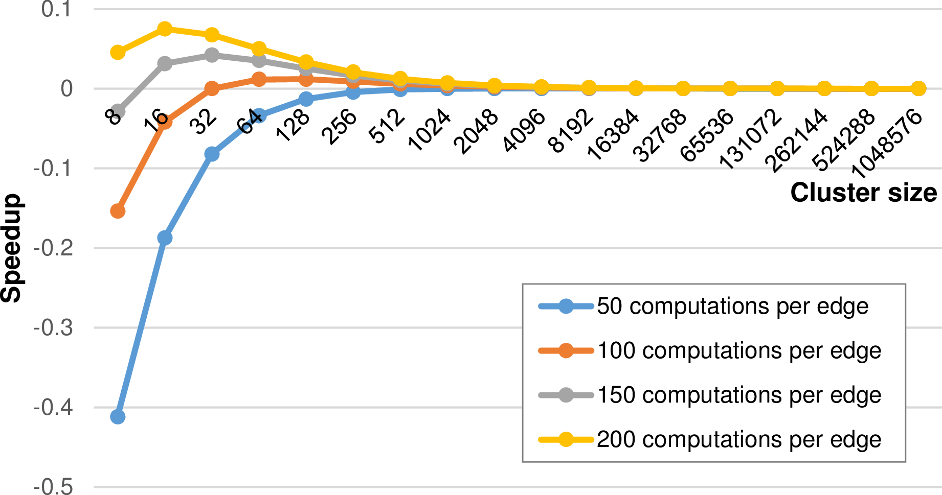
We compute the speedup using the single evaluation with  and use rule-of-thumb
values o = 1000, e.g. 1000 cycles to dequeue a task from the worker’s queue and c = 100 as the
computational workload per cell. The speedup graph for different refinement depths and thus cluster
sizes is given in Fig. 5.29 for different computational costs for edges.
and use rule-of-thumb
values o = 1000, e.g. 1000 cycles to dequeue a task from the worker’s queue and c = 100 as the
computational workload per cell. The speedup graph for different refinement depths and thus cluster
sizes is given in Fig. 5.29 for different computational costs for edges.
The shapes of our experimentally determined results in Fig. 5.28 match to our model. We find the agreement, that in case of a low computational cost involved in each edge, there’s no benefit in using a single reduce operation. For computational intensive edge reductions as it is the case for the augmented Riemann solver, using a single reduce operation can be beneficial. However, as soon as the number of cells in each cluster is getting higher, the benefits tend towards zero.
We conclude, that for small cluster sizes, avoiding duplicated reduction operations can be beneficial for small cluster, e.g. required for strong-scaling problems and the algorithm presented in the next section.
So far, we only considered adaptivity conformity traversals being executed by traversing the entire domain grid. For parallelization, we decomposed our domain with clusters and replicated data scheme to execute traversals massively parallel also in a shared-memory environment. For adaptivity traversals aiming at creating a conforming grid, the cluster approach is similar to a red-black coloring approach with information on hanging nodes possibly not forwarded to adjacent clusters in the current adaptivity traversal. Thus more traversals can be required in case of parallelization.
However, a clustering approach offers a way to compensate these conformity traversals if there are more than one clusters per compute unit: adaptivity traversals can be skipped on clusters that (a) already have a conforming grid and (b) do not receive a request of an adjacent cluster to insert an edge (adaptivity marker MR). Both requirements are discussed next:
This algorithm is based on the sparse graph representation (see Fig. 5.5 of our clustered domain: using this graph representation, our algorithm can be represented by a Petri net [SWB13a].
Algorithm: Skipping of clusters with a conforming adaptivity state
Here, each cluster is a node and the directed arcs exist for each RLE entry. Tokens represent requests for additional conformity traversals. We then distinguish between local consistency traversal tokens and adjacent consistency tokens with the latter one forwarded to, or received from adjacent clusters.
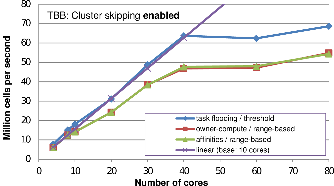
We conducted several runs for the SWE benchmark scenario from Sec. 5.7. The results are given in Fig. 5.30 with the linear scalability shown for the implementation without adaptive conforming cluster skipping. In compliance with the results for the non-skipping version, the range-based cluster generation suffers of additional overheads due to more frequent cluster generation operations. However, considering the pure task-flooding with a threshold-based cluster generation, we get a higher performance compared to the basic implementation due to algorithmic cluster-based optimizations.
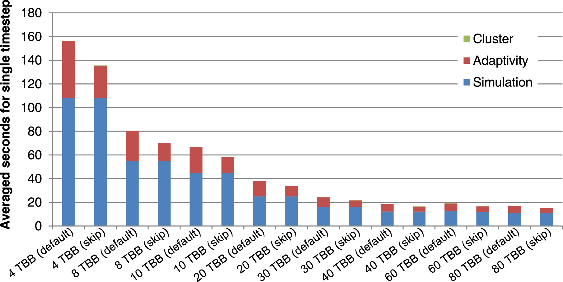
We further analyze the robustness of the adaptive cluster skipping and detailed statistics on the run time separated into the three major phases of a single simulation time step: (a) generating clusters, (b) adaptivity traversals and (c) time step traversals. The results are given in Fig. 5.31 for a different number of threads executed on the same benchmark scenario. For all tested numbers of threads, the skipping algorithm yielded a robust performance improvement. The time spent for cluster generation is negligibly small. We account for that by the required decreased time step size due to the higher-order spatial discretization. This also leads to less changes in the grid and therefore less executions of cluster generation. The presented adaptive cluster skipping also leads to robust performance improvements on distributed memory simulations, see Sec. 5.12.1.
Our run-length encoding provides an optimization for the blockw-wise data communication for stack-based communications. This section highlight the potential of saved memory storage by using our RLE meta information.
With statistics gathered for executed simulations, we compare the number of RLE-stored meta information to the number of elements required if we would store the communication primitive separately [SWB13b].
Here, we assume the meta information on vertices associated to one RLE edge communication
entry is not stored, but inferred by the per-hyperface stored edge meta information. To
give an example, we assume an RLE encoding ((A,2),(B,0),(C,3)) to be stored with
((A,e),(A,e),(B,v),(C,e),(C,e),(C,e)), see Sec. 5.2.3. We then compute the ratio between
the quantity of entries required for our RLE scheme QR := |((A,2),(B,0),(C,3))| to the
number of non-RLE encoded entries QN := |((A,e),(A,e),(B,v),(C,e),(C,e),(C,e))|. This
ratio Q :=  then yields the factor of memory saved with our RLE meta information
compared to storing the meta-communication information separately for the communication
hyperfaces.
then yields the factor of memory saved with our RLE meta information
compared to storing the meta-communication information separately for the communication
hyperfaces.
We conducted empirical tests with a hyperbolic simulation based on (a) the Euler and (b) the shallow water equations. Here, we used edge-based communication for the simulation and node-based communication for a visualization in each time step. The simulation is started with an initial refinement depth of d = 6 and up to a = 14 additional refinement levels. The simulations are initialized with the same radial dam break, using the density as the height for the Euler simulation, and we simulate 100 seconds. This resulted in execution statistics given in the table below:
| time steps | min. number of cells | max. number of cells | |
| Euler | 31 | 34593 | 40228 |
| Shallow water | 733 | 34593 | 178167 |
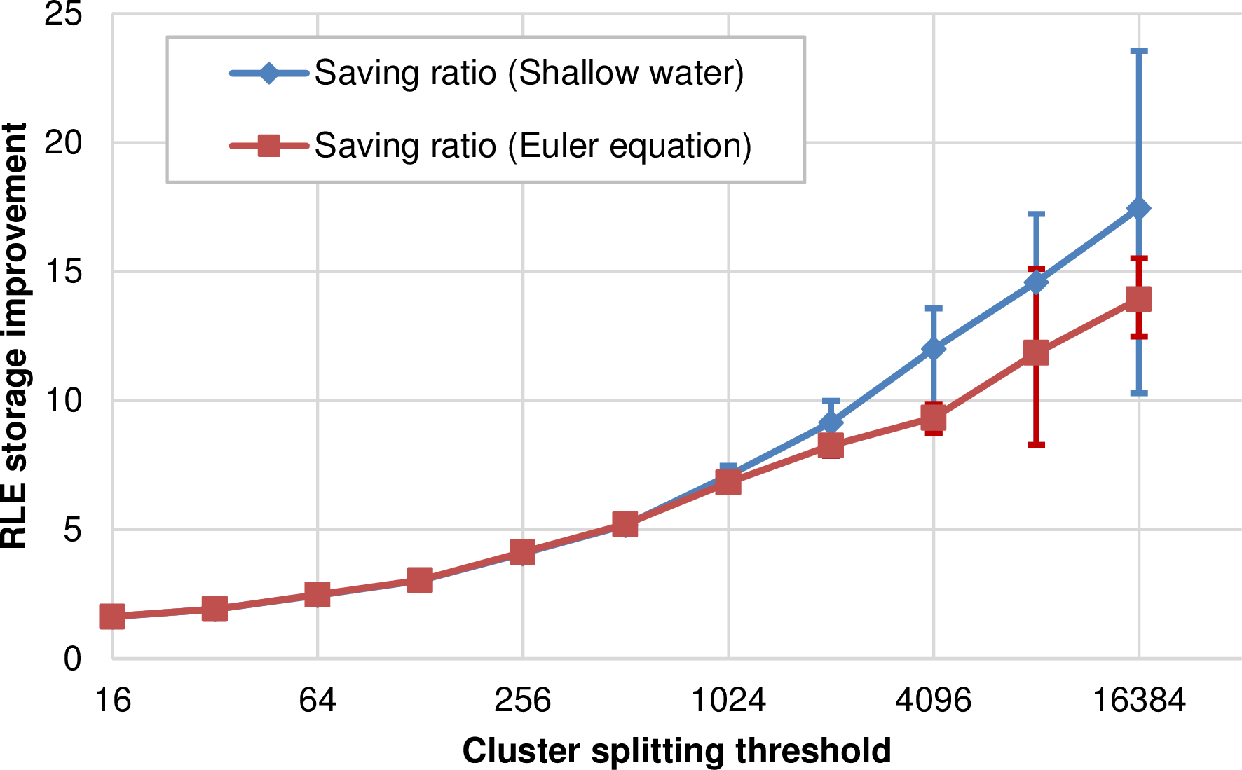
We plot the ratio Q for our simulation scenario above in Fig. 5.32. Larger clusters lead to an increased ratio due to more shared hyperfaces per cluster and hence more entries to be compressed with our RLE meta information. The min/max bounds for the largest tested cluster size with the Euler simulation is not as large as for the shallow water equation. We account for that by two statistical effects: the first one is a shorter run time which leads to less possible values involved in the min/max computation. The second one is, that less time steps for the Euler simulation also lead to less cells generated in average with a maximum of 40228 cells over the entire simulation (see the table above). This leads to only a low average number of clusters during the entire simulation, almost no dynamic cluster generation in the simulation and thus less values involved into the min/max error range. For typical cluster sizes of more than 4000 cells, the memory requirements for the meta information are reduced by factor of 9.
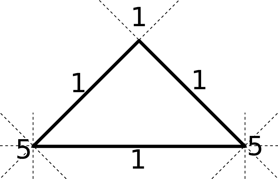
For simulations executed on unstructured grids, the meta communication information is typically stored for each cell. This is considered to be especially memory consuming for meta information on vertices due to more than a single adjacent cell compared only a single adjacent cell with edges. However, the ratio of the meta information overhead per-cell compared to our cluster-shared-hyperface RLE encoding depends on the number of degrees of freedom stored in each cell which we further analyze with a model [SWB13b]. Here, we model the payload (DoF) per cell with W and assume a regular refinement depth d, yielding 2d cells per cluster. We also assume that the non-RLE meta information takes the same amount of memory as a single DoF. Furthermore, we neglect the requirement of storing the cell orientation since this can be bit-compressed and stored in a cell requiring less storage than a single DoF. Such a cell orientation can be required if accessing the adjacent cell.
 With the grid generated by the bipartitioning Sierpiński SFC and based on our assumption of a
regular grid, the required memory for the meta information on adjacent cells for each triangle cell and
the workload for each cell are given by
With the grid generated by the bipartitioning Sierpiński SFC and based on our assumption of a
regular grid, the required memory for the meta information on adjacent cells for each triangle cell and
the workload for each cell are given by
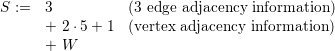
Storing the meta information only for the cluster boundaries, this yields R := 2 ⋅ (3 + 2 ⋅ 5 + 1) RLE entries to store the adjacent information with the factor 2 accounting for the two-element tuple for each entry.
The ratio of the number of cells times the memory requirements to the RLE encoded memory requirements then yields the memory saved for each cluster:

 + 1 which only depends on the per-cell payload W.
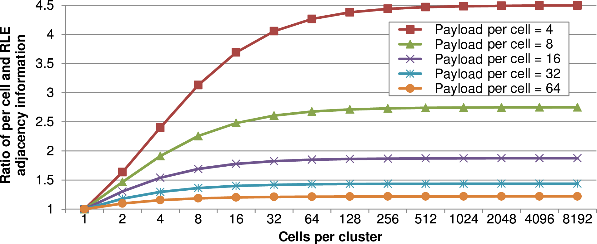
We plotted this ratio for different cluster sizes and DoF per cell in Fig. 5.33. First, this plot shows that less memory is saved for smaller cluster sizes. We account for this by clusters with less cells requiring the same amount of RLE meta information compared to clusters with more cells. Hence, for smaller clusters, the benefit of the ratio of cells to RLE encoding is getting smaller. Second, for larger cluster sizes, the plot shows the potential of memory savings for simulations with a small number of DoF per cell. According to the simplified model, this can reduce the memory consumption up to a factor of 4.5. Third, with a larger number of DoF per cell, as it is the case for higher-order simulations or by storing regular sub-grids for each cell, the benefit of our stack- and stream-based simulations with RLE meta information is below 1.5 for more than 32 DoF per cell. Though, the advantages of the RLE-based communication are still given e.g. by the block-wise communication and cluster-based data migration for distributed-memory systems (Section 5.10.3).