
So far, we presented several framework requirements and how they can be accomplished with a serial traversal of the Sierpiński SFC. This section presents several performance improvements with hardware optimizations and algorithmic developments.
Stack push and pop operations depend on the edge (Section 4.3.3) or vertex types (Section 4.3.4) as well as the order in which they are accessed (Section 4.3.2). A straightforward implementation would lead to inheritance of such types and utilizations of if-branchings for distinguishing between whether a push or pop operation has to be done as well as on which stack such an operation has to be executed.
We only consider new and old edge types without loss of generality and start by describing the issues with the non-optimized version: For different if-branches used to distinguish between these two edge types, a typical branch prediction would lead to a miss rate of 50% in average. We expect this to lead to less performance due to discarding instructions in the pipeline and thus reduced efficiency for the grid traversal.
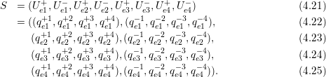
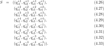
With our code generator (Section 4.9.5), we can consider the recursive spacetree traversal code be given by

We compared grid traversals with and without parameter unrolling on an Intel(R) Xeon(R) CPU X5690 with 3.47GHz. A regular grid resolution with 22 refinement levels is used with 12 floating point operations in each cell. The vertices are computed during the grid traversal on-the-fly.
On the one hand, this leads to increased size of machine code and therefore a severely increased instruction cache miss rate by a factor of 33.7. On the other hand, the if-branching mispredictions are reduced by a factor of 4.7 in average. Having a look at concrete runtime results shows that the avoidance of if-branching mispredictions outperforms the increased instruction cache misses:
| parameter unrolling | with parameters | performance increase | |
| GNU Compiler | 5.066 sec | 6.044 sec | 19.3% |
| Intel Compiler | 3.806 sec | 5.130 sec | 34.8% |
Hence, such an optimization is important for kernels with only a few operations.
Due to the recursive grid traversal, we should be aware of the overhead of recursive methods. This overhead involves calls of our methods as well as the parameter handling of the methods. Therefore, kernels and traversal methods are prefixed with the inline statement, instructing the compiler not to use a function call to this method but to inline the code of the method directly. This aims at avoiding function calls. Similar inline optimizations are also used for the stack and other core operations.
With the adaptivity traversals presented in Section 4.6, a single traversal only considers the change of adaptivity state, but not the direction of propagation of the adaptivity markers.
In case that a refinement marker is forwarded via an edge and the traversal direction propagates this information to the adjacent cell within the same traversal, this assures the processing of the refinement marker within the same traversal. Thus forwarding and processing the refinement marker in the same traversal is assured for edges of type new. If all refinement markers can be forwarded in the traversal, also the grid is assumed to be in conforming state.
| incoming edge marker
| |||||||||
| state t | 000 | 001 | 010 | 011 | 100 | 101 | 110 | 111 | |
| no request | 0 | 000,0 | 100,5 | 100,6 | 100,7 | 000,4 | 000,5 | 000,6 | 000,7 |
| INVALID | 1 | 000,1 | 000,1 | 000,1 | 000,1 | 000,1 | 000,1 | 000,1 | 000,1 |
| local coarsening req. | 2 | 000,2 | 100,5 | 100,6 | 100,7 | 000,4 | 000,5 | 000,6 | 000,7 |
| local refine request | 3 | 100,4 | 100,5 | 100,6 | 100,7 | 000,4 | 000,5 | 000,6 | 000,7 |
| refined: hyp | 4 | 000,4 | 000,5 | 000,6 | 000,7 | 000,4 | 000,5 | 000,6 | 000,7 |
| refined: hyp, left | 5 | 000,5 | 000,5 | 000,7 | 000,7 | 000,5 | 000,5 | 000,7 | 000,7 |
| refined: hyp, right | 6 | 000,6 | 000,7 | 000,6 | 000,7 | 000,6 | 000,7 | 000,6 | 000,7 |
| ref.: hyp, right, left | 7 | 000,7 | 000,7 | 000,7 | 000,7 | 000,7 | 000,7 | 000,7 | 000,7 |
We construct an automaton with initial states given by the adaptivity states, transition states based on the adaptivity markers read via edge communication and remaining adaptivity markers to be forwarded. This automaton can be written in a tabular format (see Table 4.1) and is used as follows.
Each grid cell has its own adaptivity state S := (f,t) which consists out of the refinement information which still has to be forwarded via each edge in a bit field f := {0,1}3 for edges (e1,e2,e3); t represents one of the adaptivity states from (0) to (7).
Considering refinement operations only, the transition function is then based on a table lookup using the current adaptivity state f selecting the row and the input bit fields storing the incoming edge markers selecting the column in Table 4.1. The new state of a single cell is then given by the entry (f,t) of the table cell. Bits set in fupdate represents the required refinement information which still has to be forwarded via edges.
Based on the current transition state (f,t), the tuple of the refinement requests t to be forwarded to adjacent cells and the new transition state can be determined via a lookup in the automaton table with the current incoming refinement requests T, yielding (fupdate,tnew).
In case of a cell transition set to coarsening (2), the propagation of the coarsening agreements marker MC is immediately stopped in case of an incoming marker fetched via a cathetus is not of type MC.
Forwarding of refinement information: Since the information to be forwarded is already included in f, required refinement markers are also stored in fupdate. A bitmask is used with bits set for edges of type old. This bitmask is ANDed to f to account for edges of type (a) new with refinement information propagated during the current cell traversal and (b) boundary which do not require forwarding of refinement information.
This adaptivity automaton is able to avoid at most one traversal for serial traversals. However it turns into a crucial component for the optimization with the cluster skipping approach in the parallelization (See Section 5.8.2).
With the trend of computing cores requiring operations on data stored in vectors to get close to the peak of floating point operations, utilization of vector instructions is mandatory for HPC-oriented developments.
Regarding the flux computations on the edges for higher-order DG simulations, multiple nodal points for flux evaluation are available on each edge. This allows a straightforward optimization with SIMD operations.
For 0th-th order discretization, however, only DoF of a single node on the edge is stored per edge. Here, SIMD optimizations are still possible for a pair of nodal points e.g. by computing multiple square roots in the Rusanov solver with a single SIMD operation.
In this section, we like to focus on an alternative method for 0th-th order discretizations. We consider, that the nodal-wise given conserved quantities are stored consecutively on the edge buffer stacks. 4 Since the DoF on the edge buffer stack are stored in the format of arrays of structure and since SIMD operations typically demand for a structure of arrays, the data has to be rearranged. We consider a block of multiple conserved quantities Ui+,Ui- for the left and right state of an edge stored to the edge buffer stack:
As a proof of concept, we conducted benchmarks based on the augmented Riemann solver [Geo06] which were SIMD optimized in [Höl13]. In this work, the SIMD-optimized augmented Riemann solver is implemented with single precision. We compare the SIMD performance improvements with this solver based on simulations with a radial dam break szenario. The simulation is executed with an initial refinement depth of d = 16 and with a = 10 additional levels of adaptive grid refinement. The SIMD optimization which we used for the benchmarks stores 4 single-precision components in each vector, and we execute the simulation for 100 time steps.
We measure the optimization for the edge communication and adaptivity traversal times given in seconds:
| SIMD disabled | SIMD enabled | |
| Time step | 10.86 | 6.66 |
| Adaptivity | 3.99 | 3.93 |
The time to compute a time step is improved by 38.7% but the maximal theoretical improvement of 75% was not reached. We account for that by (a) the branch divergence inside the flux solver resulting in non-parallalelized sections and (b) the grid traversal time which was not optimized with the SIMD flux evaluation. The runtime for the adaptivity traversals is not reduced since the SIMD optimized solvers are only used in the time step traversals.
Considering the flux computations of conserved quantities with higher-order basis functions (see Section 2.3), we can use SIMD instructions by storing the weights for the basis functions in a structure of arrays. We store the n weights qji with j ∈{1,…,n} for a particular conserved quantity i of a cell consecutively in memory. For four conserved quantities, this yields

In this work, we followed this structure-of-arrays format for our conserved quantities, however, we did not further focus on optimization of such matrix-matrix computations.
A straightforward implementation of the stack system with the C++ std::vector class from the standard library would lead to a performance slowdown: an obvious example is given by frequent memory free() and alloc() operations if not pre-allocating sufficient memory and thus re-utilization of already allocated memory. Pre-allocating far more memory than required leads to a severe additional memory consumption, possibly exceeding the available memory.
With a prospective stack size allocation based on an upper limit for the maximum required allocated stack, we can overcome testing for exceeding stack access and avoid any stack resize operations during grid traversals. Using the knowledge on the number of cells c (See [Vig12]) for our simulation domain assembled by a triangle, upper limits for the storage requirements on all stacks can be determined. The number of cells c after all adaptivity traversals on a grid can be derived based on the adaptivity state information before updating the grid structure. The number of grid cells are increased for each inserted edge and decreased for a pair of coarsening requests stored on the adaptivity state stack. See e.g. Fig. 4.8 with the red-dashed lines representing the inserted edges for the refinement operations (3) to (7).
Here, we infer the upper limits of the required stack storage:
The cell data stack size is directly set to c.
An upper limit of the size of the structure stack is directly given by the recursive structure. With a cell split achieved by replacing 0 with 100 on the structure stack, this creates 2 additional bits for each new cell. Starting with a single cell represented by a stack storing |0 only, i.e. only one entry, this yields

Edge communication data such as SsimEdgeComm for running the simulation or SadaptiveEdgeComm for adaptivity traversals is limited by recursive bisection of the communication edges. We follow a greedy approach successively splitting triangles targeting at creating as many edges as possible at the triangle boundary at the root spacetree node. This leads to a sequence of maximum edge communication elements E with Ei representing the upper limit of required stack storage for the i-th inserted edge. For the right communication stack, this yields Eright := (1,2,2,3,3,4,4,5,5,6,6,…) and Eleft := (2,2,3,4,4,5,5,6,6,7,7,…) for the left communication stack. With Ei := max(Eileft,Eiright) = Eileft, an upper limit is given by

 ) + 2.
For the root triangle, at least six edge buffer elements are required due to storing up to six boundary edge data elements on the buffer stacks. With each refinement of child triangles, two additional edges are created for the shared edge and two additional edges are created due to splitting the edge on the hypotenuse. This demands for additional storage of four elements on the stack system. Thus, the maximum number of required edge buffer data for edge data is

For vertex data, only two nodes can be stored on each communication stack. Following a greedy edge insertion focussing on creating as many vertices as possible on the boundary of the domain created by the spacetree, this yields


For the visualization, the vertex buffer only requires data storage for the vertices inside the domain since the boundary vertex data is stored to the vertex communication stacks. Each insertion of an edge creates one additional vertex. Since those inner vertices can be created only with more than 4 cells and one additional vertex is generated for each new cell, this yields:

We derived maximum stack size capacities to store all data during a traversal based on a given number of simulation cells c. This new snumber of simulation cells was derived with the adaptivity state flags on the stack after the conforming adaptivity state was detected.
Before the last backward adaptivity traversal, we then reallocate the output stacks with the new capacity. The other stacks are reallocated after the last backward adaptivity traversal. This avoids resize operations during all traversals.
However this would still yield a frequent reallocation of stack data if the number of cells changes. Therefore, we introduce two additional padding values: Ppadding and Pundershoot. These thresholds are applied in case of exceeding and undershooting a particular number of simulation cells.
A reallocation is done only if |SsimCellData| < c or |SsimCellData|-Pundershoot > c. This reallocates the stacks for c + Ppadding simulation cells.