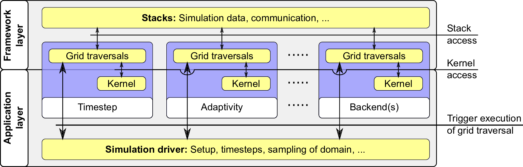
Figure 4.12: Overview of the serial framework design.
Using the introduced communication via stacks and streams, no direct access of adjacent primitives is possible2 . Also implementing SFC grid traversals with a stack- and stream-based approach, a solution was already suggested in the Peano framework [Wei09]: the application developer has to implement a kernel with the grid traversal calling corresponding kernel methods. However, this framework uses only interfaces for vertices and cells whereas we require additional access to e.g. semi-persistent edge- and node-based data. Therefore, we follow a similar software concept compared to the one of the Peano framework for the vertices and introduce additional interfaces as well as additional framework considerations. The building blocks used for the software design, capable of running single-threaded simulations, are given in Fig. 4.12.
For the application layer, we follow the concept “what to do rather than how to do it” from Intel’s Array Building Blocks [NSL+11]. With a kernel-based software design, the framework user thus specifies what to compute on the grid rather than how to traverse and access the grid data.
Framework layer: How to access grid data and how to store grid and communication data is based on the stack- and stream-based approach presented in the previous Sections. Which data is associated to grid primitives and in which way these are accessed (see Section 4.4 on classification of stack data access) typically depends on the simulation requirements and, thus, is only known and has to be specified by the application developer. “How to” manage the data stored on the grid and to hide the way how it is accessed is then the task of the framework layer. “What to do” with the data offered by the framework layer then has to be specified by the application developer.
Application layer: Based on the framework layer providing access to the grid data, the application developer then specifies operations to this grid data in the kernels.
Starting grid traversals and corresponding operations on grid data is initiated by the simulation driver. Such traversals can be the simulation time step itself, traversals for adaptivity, writing simulation data to permanent storage using backends, etc. This driver is either implemented by the application developer or provided by a default driver from the framework.
Grid traversals manage the data access by executing push and pop operations on stacks. These operations depend on the data access demands specified by the application developer. The data references are then forwarded to the kernels to store, update or read the data which is managed by the grid traversal.
For efficiency reasons, we use specialized kernel interfaces based on the grid data access requirements instead of providing all possible grid data accesses, leading to data management overhead in the case that obsolete data is accessed (e.g. if no vertex data is required) or has to be generated. To give an example, vertex coordinates are not required for mid-adaptivity traversals. Next, we describe how to specify the specialized kernel interfaces.
We can specify the grid data access relations of a single traversal in a matrix. This matrix
relates the input (row) and output (column) relations between data stored at grid primitives
 := {cell,edge,vertex,adaptiveState}. The additional adaptivityState is required for the adaptivity
state information used by the adaptivity traversals and is stored on an additional stack
structure.
:= {cell,edge,vertex,adaptiveState}. The additional adaptivityState is required for the adaptivity
state information used by the adaptivity traversals and is stored on an additional stack
structure.
A single forward or backward traversal can then be represented with the matrix  (a,b) with
a,b ∈ describing the operations executed on data associated to the cell primitives. Then each
matrix entry describes the standard grid data access type (persistent, creating, clearing, see
Section 4.4).
(a,b) with
a,b ∈ describing the operations executed on data associated to the cell primitives. Then each
matrix entry describes the standard grid data access type (persistent, creating, clearing, see
Section 4.4).
We give an example for the forward traversal of the simulation which computes the flux parameters. Here, we can specify the kernel interface requirements with the following matrix and only include columns and rows which are relevant:
| Output
| |||
| cell | edge | ||
|
Input | cell | flux creating | |
| edge | |||
Whereas these matrices account for accessing the grid data itself, further kernel parameters can be e.g. cell vertices and cell normals which are computed during the grid traversal on-the-fly. Such kernel parameters are computed during the grid traversal and are not stored in each cell to reduce the bandwidth requirements. We can optimize grid traversals without any requirements of such kernel parameters by avoiding computations of obsolete kernel parameters during the traversal. E.g. traversals such as the middle adaptivity traversal only update the adaptivity state information and do not require cell’s vertex coordinates and normals.
Furthermore, we restrict the kernel interfaces for accessing grid data to one or two grid primitives. Hence, interfaces such as storing cell-based data to a vertex and to an edge are not allowed. Those interfaces are described by
![c1[xtoxc2[xP ]](parameters)](schreiber14dissertation118x.png)
For our DG simulation, we use this interface type to update the conserved quantities stored in each cell (c1 = {cell}) based on the computed fluxes stored on edges, {edge1,edge2,edge3}∈ parameters.
For the visualization tasks, such a type of kernel function is also used to generate the triangle data to be used for visualization, based on vertex data, {vertex1,vertex2,vertex3}∈ parameters
In the case that c1 = c2, this accounts for updating the data stored on both primitives. This is e.g. used for edges to compute the fluxes after storing the DoF to the edge buffers.
 ]](parameters){…}: (see Sec. 4.3.4) differentiating
between first-, middle- and last-touch operations.
]](parameters){…}: (see Sec. 4.3.4) differentiating
between first-, middle- and last-touch operations.
These interfaces are then used for the visualization to store the DG surface data to vertex primitives c2 = {vertex1,vertex2,vertex3}.
For the parallel implementation, additional framework interfaces are used for the synchronization of the replicated shared interfaces with only partly updated data.
All the possible parameter combinations discussed in the previous section lead to a manifold of grid traversal variants.
Creating different optimized kernels using template features of C++ allows for a modification of particular features and requirements of grid traversals; however, it does not allow for the modification of the number of parameters e.g. to disable computing vertex coordinates forwarded via parameters during recursive grid traversal.
As previously mentioned, we decided to create grid traversals using a code generator and discuss it here in more detail. This generator creates optimized code for the grid traversal which is tailored to the grid traversal requirements based on the knowledge of the application developer.
Configuration parameters for this generator besides T (see Section 4.9.4) are e.g.
For efficiency reasons, vtable calls have been avoided for the interfaces by inheriting a kernel class to the grid traversal class since overhead optimizations of such vtable calls mainly depend on the used compiler.
For a forward DG simulation traversal storing fluxes, we get
| Output
| |||
| cell | edge | ||
|
Input | cell | flux creating | |
| edge | |||
with flux clearing as a special tag to create specialized code for flux computations. For the backward traversal the matrix is given by
| Output
| |||
| cell | edge | ||
|
Input | cell | ||
| edge | flux clearing | ||
for executing cell operations with fluxes (edge data) as input.
We can then implement the first adaptivity traversals with
| Output
| ||||
| cell | adaptiveState | edge | ||
|
Input | cell | creating | non-persistent | |
| adaptiveState | ||||
| edge | ||||
thus computing the adaptive state based on cell-wise stored data and forwards adaptivity markers via edges. In case that the adaptivity state flags were created during the backward traversal of the simulation time step, we can skip this forward traversal and start directly with the middle adaptivity traversal.
The middle adaptivity traversals are required to assure a conforming grid and are specified by
| Output
| |||||
| cell | adaptiveState | edge | |||
|
Input | cell | ||||
| adaptiveState | persistent | non-persistent | |||
| edge | |||||
This operates on the adaptive state flag only. Thus, no access of simulation cell data is required.
Finally, a last backward traversal refines and coarsens cells depending on the adaptivity state flags while still transferring adaptivity markers along edges. This transfer is required to transfer coarsening “disagreement” information to adjacent cells in case of no middle traversal. Otherwise, this can lead to a coarsening which creates a hanging node. Furthermore, the last adaptivity traversal is specially tagged to execute kernel methods to compute the DoF of the refined or coarsened cells.
| Output
| |||||
| cell | adaptiveState | edge | |||
|
Input | cell | persistent | |||
| adaptiveState | clearing | (non-persistent) | |||
| edge | |||||
Presistent cell data is updated (refine or coarsen cells) and the adaptive states are cleared from the stacks. Creating non-persistent adaptivity information on the edges is an important component for the meta communication information used for our parallelization which is discussed in Section 5.2.3.
To show the applicability of our vertex-based communication, we compute the vertex data based on the data stored in each cell. This results in the following communication matrix
| Output
| |||
| cell | vertex | ||
|
Input | cell | creating | |
| vertex | non-persistent | ||
which computes the vertex data based on cell-wise stored DoF. Here, the non-persistent vertex access type is implemented with a reduce operation on each vertex. The backward traversal is then given by
| Output
| |||
| cell | vertex | ||
|
Input | cell | ||
| vertex | clearing | ||
finally assembling the vertex information for each cell.