 and
and  and
and With a simulation on a dynamically adaptive grid, we refine and coarsen our cells during runtime by splitting triangles into two triangles and merging them respectively. Then, the conserved quantities require projection to the refined or restricted grid cells.
We start by determining a way to compute the coefficients of the approximating solution on our reference triangle based on the weights of given basis functions. This also leads to computations of the weights of the basis functions from a given approximating solution.
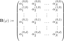
We start by denoting the coefficients of the monomials which assemble the basis polynomials (see Section 2.3) φi(x,y) := ∑ (a,b)αi(a,b)xayb, with αi(a,b). Here, it holds that 0 ≤ a + b ≤ d, 0 ≤ a and 0 ≤ b. We construct a d × n coefficient matrix

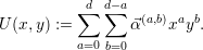
 represent the coefficients of the monomials of our approximated
solution φ(x,y) := ∑
iqiφi(x,y).
represent the coefficients of the monomials of our approximated
solution φ(x,y) := ∑
iqiφi(x,y).
In case of only one conserved quantity, we are now able to compute the coefficients of the polynomial related to our approximating solution
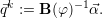
We use this matrix formulation for computing the basis function weights  k of the
basis functions for a given approximating solution by inverting the coefficient matrix B(φ),
yielding
k of the
basis functions for a given approximating solution by inverting the coefficient matrix B(φ),
yielding
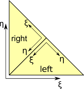
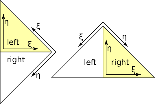
Due to splits and joins, a transformation of the DoF to and from different triangles is required, see Fig. 2.5. We respectively denote the triangle space which is split as the parent triangle space and both split ones which have to be possibly joined as the children triangle spaces.
Let
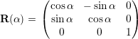 | (2.19) |
be a two-dimensional rotation matrix computing rotations in clockwise direction for positive α,
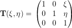 | (2.20) |
a translation matrix and
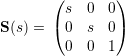 | (2.21) |
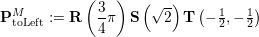
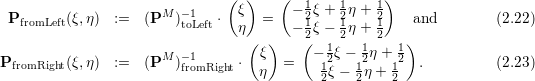
a scaling matrix. A transformation matrix returning the sampling point in the child’s left reference space if sampling in parent reference space is then given by
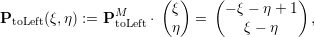
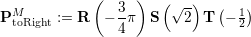
For the right reference triangle, this yields
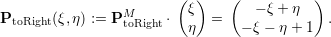
Sampling of the child’s approximated solution using reference coordinates from the parent reference space then gives

By using a representation of the child’s basis functions in parent’s reference space, the refinement matrix is determined by first computing the polynomial coefficients for the approximating polynomial in parent space with B(φ) and then reconstructing the weight qk for the child’s polynomials by using the representation of the child’s polynomials φ
toLeft(ξ,η) in the parent space:
Restriction operations can be computed in a similar manner to the prolongation (see Eq. (2.25)). However, due to the discontinuity at the shared edges of the children, the approximated solution of both children cannot be represented by a single parent triangle.
We choose a restriction which is averaging the polynomial basis functions of both children extended to the parent’s support yielding

 | (2.27) |
Such an averaging is obviously not able to reconstruct the polynomial accurately in case of discontinuities at the shared edges as this is typically the case for our DG simulations. We want to emphasize, that other coarsening computations, e.g. reconstructing the basis polynomial with minimization with respect to a norm, can yield improved results. With improved reconstruction methods being transparent to the determined interface requirements and since this section focuses on the determination of the basic requirements for the computation of DG-based simulations, we continue using this coarsening method.
The derived restriction and prolongation matrices can be applied transparently to either nodal or modal basis functions since their construction is based on the coefficient matrix, which is again based on the coefficients of the basis polynomials.
To trigger refining or coarsening requests on our grid, we use error indicators to distinguish between refining, coarsening or no cell modifications.
For this work, we considered two different adaptivity indicators:
If an indicator exceeds a particular refinement threshold value, a split of the cell is requested. In case of undershooting the coarsening threshold value, the indicator allows joining this cell with an adjacent one in case of both cells agreeing in the coarsening process.
