6.1 Prerequisites

Before running benchmarks with the shallow water equations, we need (a) solvers with the capability of running accurate simulations, (b) an error norm for objective statements on the accuracy, (c) an error indicator to trigger refinement and coarsening requests, and (d) an extension of the refinement and coarsening operations due to bathymetry. These issues are briefly addressed in the upcoming sections.

6.1.1 GeoClaw solver

For a correct handling of wave propagations, we decided to use the augmented Riemann solver from the GeoClaw package [Geo08,BGLM11]. This solver is well-tested in the context of shallow water and Tsunami simulations [MGLT] and operates on the cell averaged conserved quantities (h,hu,hv,b), respectively the distance of the water surface to the bathymetry, the momentum in x-direction, the momentum in y-direction and the bathymetry relative to the horizon. Using the augmented Riemann solver, the flux computations with the adjacent cells are replaced by solvers computing so-called net updates. These solvers compute the net flux from one cell to another one.

Then the conserved quantities are directly improved based on the computed net updates for h, hu and hv and we use the b variable to store the wave speed for the accurate computation of the time-step size. For usability issues, we reuse the reference space (see Sec. 2.2) and the same framework interfaces as for the higher-order simulation.

6.1.2 Error norm

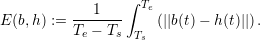
In the following benchmarks, we require an error norm for an objective comparison of simulations conducted with different parameters. We followed the suggestion in [RFLS06] to use the L1 error norm on the surface heights over time for shallow water simulations. However, instead of using the relative error, we decided to use the absolute error to avoid any influence in the computed error induced by our adaptively changing bathymetry. Let the interval to compute the error be given with t ∈ [T_s,T_e]. The L1 norm is then applied to the absolute difference of our computed solution h(t) to the baseline b(t):

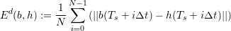
With a given data set at discrete sampling points for comparison with our baseline, we use spline interpolation and compute equidistantly distributed sampling points which are then used to compute the error with E^d. We chose the number of equidistant sampling points to a robust value which does not lead to significant changes in the computed error norm (typically larger than 20000).

6.1.3 Error indicator

With our main focus on computing the solution within given error bounds as fast as possible, only grid cells with a particular contribution (feature rich areas) to the final result should be refined. We implemented two different adaptivity criteria, each one strictly depending on the per-cell stored data to avoid additional edge-communication data.

• Horizontal deviation:
  This adaptivity criterion is based on the absolute value of the water surface deviation from the horizon, yielding with b the bathymetry which is negative for the sea ground and h the water surface distance to the bathymetry.

  This error indicator does not consider the size of the cell and is therefore unaware of the refinement depth. This would result in possible refinement operations up to the maximum of the allowed refinement depth.

• Net-updates:
  With net-update-based solvers, we can use an error indicator based on the net-update component Δh which represents the amount of fluid streamed over an edge with a unit length and a unit time-step size. We use this to determine a steady state with respect to the water surface elevation. In case that as much water is flowing into the cell as it is flowing out (i.e. a balanced state), the amount of fluid in a cell is not modified. This yields the following adaptivity criteria for the per edge communicated net-update components Δh_i: with |e_i| the length of the triangle edge i.

  This error indicator is based on the edge length and is therefore sensitive to the refinement depth.

Then, each cell requests a refinement operation in each time step in case of I > α

refineandthecellagreestocoarseningincaseofI ¡ α

coarsen.

For the benchmark studies in the following chapter, only the net-update based simulation was successfully applied to improve the computational time with dynamically adaptive mesh refinement for the considered simulations. Therefore, we restrict the presentation of our results to these indicators. We like to emphasize, that this does not induce, that the height-based adaptivity criteria cannot be used for efficient dynamic adaptive grids, but that our considered parameters did not yield satisfying results.

Alternative error indicators are e.g. based on the derivative of the surface height [RFLS06] and require additional data transfers via edges. With the focus of our studies on justification of the dynamically adaptive grids and since we will see that our results already justify the dynamical adaptivity, we did not further investigate alternative error indicators.

A final remark is given on the net-update-based error indicator: we expect, that this indicator cannot be applied to flooding and drying scenarios since the water surface height close to the shoreline tends towards zero. Hence our error indicator does not lead to refining the grid in this area. Since the sampling points in our considered scenario are in a simulation area with a relatively deep water compared with the average depth, a modification of the net-update-based solver for flooding and drying scenarios, e.g. by dividing it with the average depth of the cell, was therefore not required.

6.1.4 Refinement and coarsening with bathymetry

In contrast to the previous shallow-water test scenarios, the scenarios from the following section have a non-constant bathymetry value. Due to refinement and coarsening operations with our dynamically adaptive grid, we require an extension for the refinement and coarsening operations for the conserved quantities including bathymetry.

We discuss the conservation schemes based on the conserved quantities U := (h,hu,hv,b) and denote the conserved quantities in the parent cell with U_p and for both children with U_1∕2. We determine the bathymetry data b_1∕2 by sampling the bathymetry data set at the cell’s center of mass.

We further assume that the water surface should stay on the same horizontal level after a refinement operation to avoid spurious gravitation-induced waves. We can assure this by initializing the water height for both cells with

With the velocity of the moving wave being one of the most important features for wave-propagation dominated schemes, we used a velocity conserving scheme: We compute the velocity of the parent cell with u_p := , v_p := and initialize the momentum of each child cell with (hu)_1∕2 := h_1∕2u_p, (hv)_1∕2 := h_1∕2v_p, respectively. The coarsening operation uses the averaged velocity of both joined cells to reconstruct the conserved quantities in the parent cell.

Using the velocity conservation yielded the best results for our simulations executed in the ongoing sections. Alternative approaches such as conserving the momentum resulted in less stable simulations and were thus not further considered.