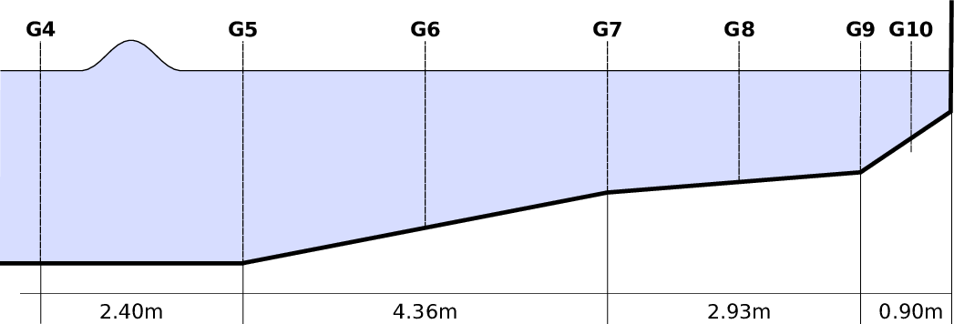
Figure 6.1: Scenario sketch for the solitary wave on composite beach benchmark.
We selected the Solitary Wave On Composite Beach (SWOCB) benchmark of the NOAA1 benchmarks which is suggested for Tsunami model validation and verification2 to show the correctness and applicability of the run-time adaptivity of the developed framework in the context of an analytic benchmark. Despite its complex simulation scenario with non-constant bathymetry, there is an analytical solution available [UTK98] which makes this benchmark very interesting. Acknowledgement: This benchmark was implemented in collaboration with Alexander Breuer.
We use scenario A of the benchmark, with a sketch of its scenario given in Fig. 6.1. This
benchmark is based on a wave which is first moving over a bathymetry with a constant depth of 0.218
and then entering an area with three non-constant bathymetry segments, with a slope of  ,
,  , and
, and
 respectively.
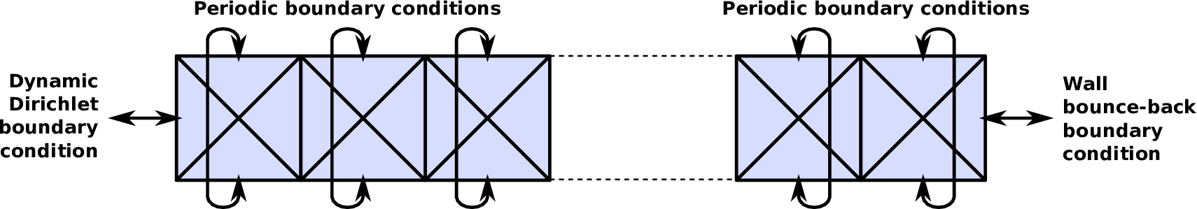
Three different boundary conditions are required (see Fig. 6.2). We set the wall boundary condition on the right side of Fig. 6.1 to bounce back boundary conditions (see Sec. 2.11.3). The boundaries on the scenario sides (top and bottom side in Fig. 6.2) are set to be periodic conditions, thus simulating an infinitely wide scenario. For the input boundary condition on the left side with the wave moving in, we do not model the initial wave form and its momentum, but use the boundary conditions of the analytical solution from the GeoClaw group provided via the git repository3 .
With our framework, we can setup such a geometry by assembling the domain with a quadrilateral strip where each one is assembled by four base triangles, see Fig. 6.2. Due to our requirement of uniquely shared hyperfaces (see Theorem 5.2.2), we are not allowed to assemble a quadrilateral by only two triangles, since this would lead to the same adjacent cluster in the RLE meta communication information for the left and right communication stacks. Therefore, we used four triangles to assemble a quadrilateral, circumventing this issue for edge communication. We initialize the domain with a strip of 128 quadrilaterals, hence resulting in 29 initial triangles for refinement depth 0. Then, for initial refinement depth d, the domain is initialized with 2(9+d) triangle cells.
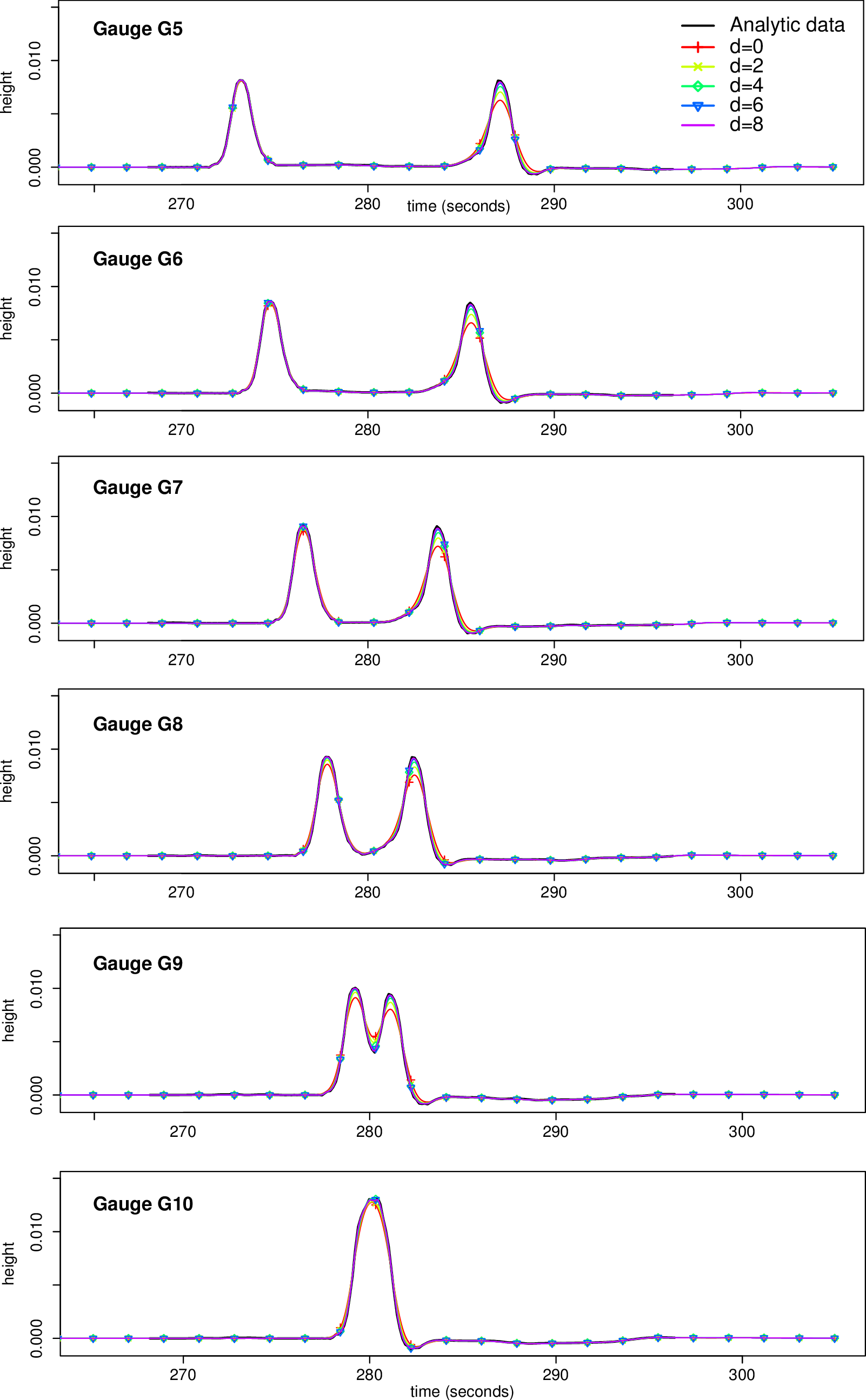
We first analyze the approximation behavior with different regular refinement depths without the dynamic adaptivity enabled. The plots for water surface height at different water gauge stations G5 - G10 are given in Fig. 6.3. We can see
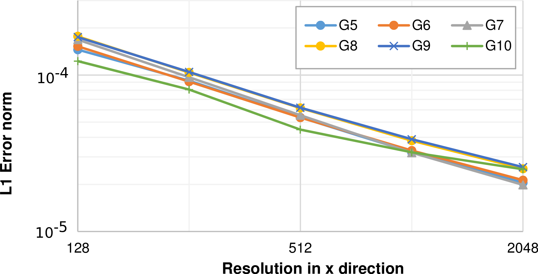
A more detailed analysis of the convergence error based on the L1 norm with the analytic solution (see Sec. 6.1.2) is given in Fig. 6.4 for all water gauge stations. This is based on the L1 error norm computed over the interval [270,295] and is decreasing for higher resolutions.
Next, we select water gauge G8 for testing the possibilities of dynamic adaptivity based on the L1 error norm computed for this gauge station. We executed several parameter studies with the initial refinement depths d ∈{0,2,4,6,8} and additional adaptive levels a ∈{0,2,4,6,8} with the constraint d + a < 8. Hence, we do not allow any spacetree depths exceeding 8.
A good justification for dynamic adaptivity is to show improved accuracy results with less cells involved in the computation. Following this idea, we executed the benchmark on a regular grid with d = 6, yielding 29+6 = 32768 grid cells, computed the error norm (6.1.2) resulting in an error of 3.80e–5 and use this as a baseline for comparison with simulations on dynamically adaptive grids.
We execute the benchmark studies within the set of allowed d and a parameters described above
and compare the results using the net-update-based error indicators (see Sec. 6.1.3). The refinement
adaptivity parameter was chosen as r := 10-n with n ∈ ℕ and the coarsening paramter in a very
conservative manner with c :=  . For a better overview, we only focus on simulations yielding
improved L1 error norm results compared to our baseline. The cell distribution over time for these
simulations is plotted in Fig. 6.5.
. For a better overview, we only focus on simulations yielding
improved L1 error norm results compared to our baseline. The cell distribution over time for these
simulations is plotted in Fig. 6.5.
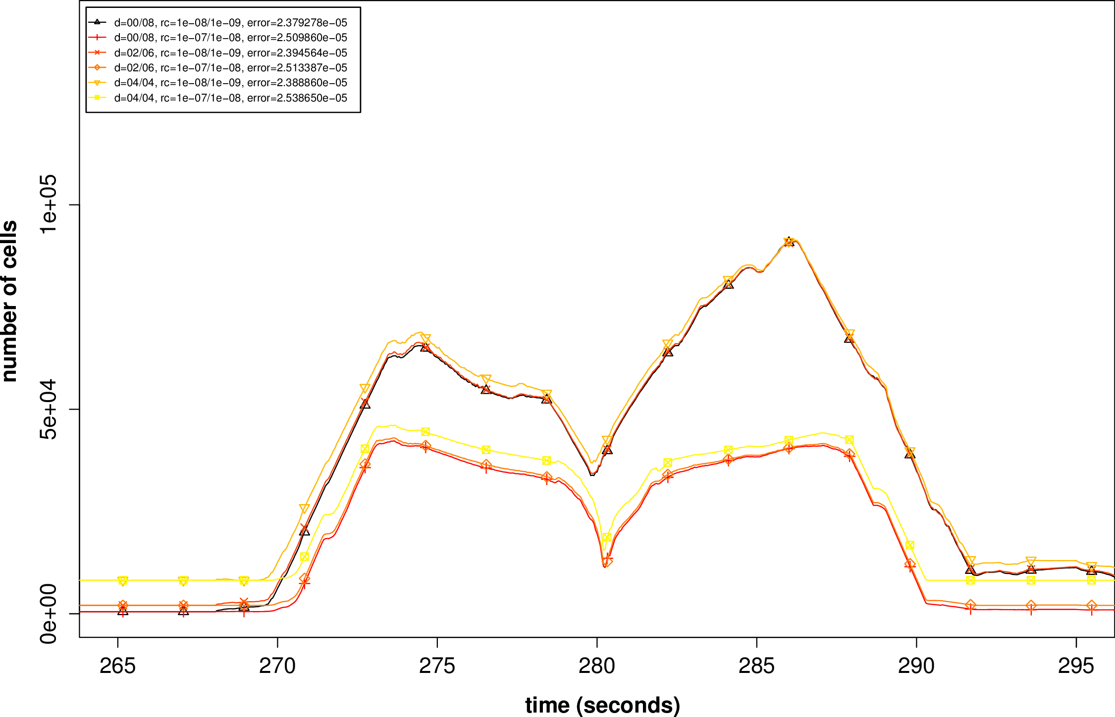
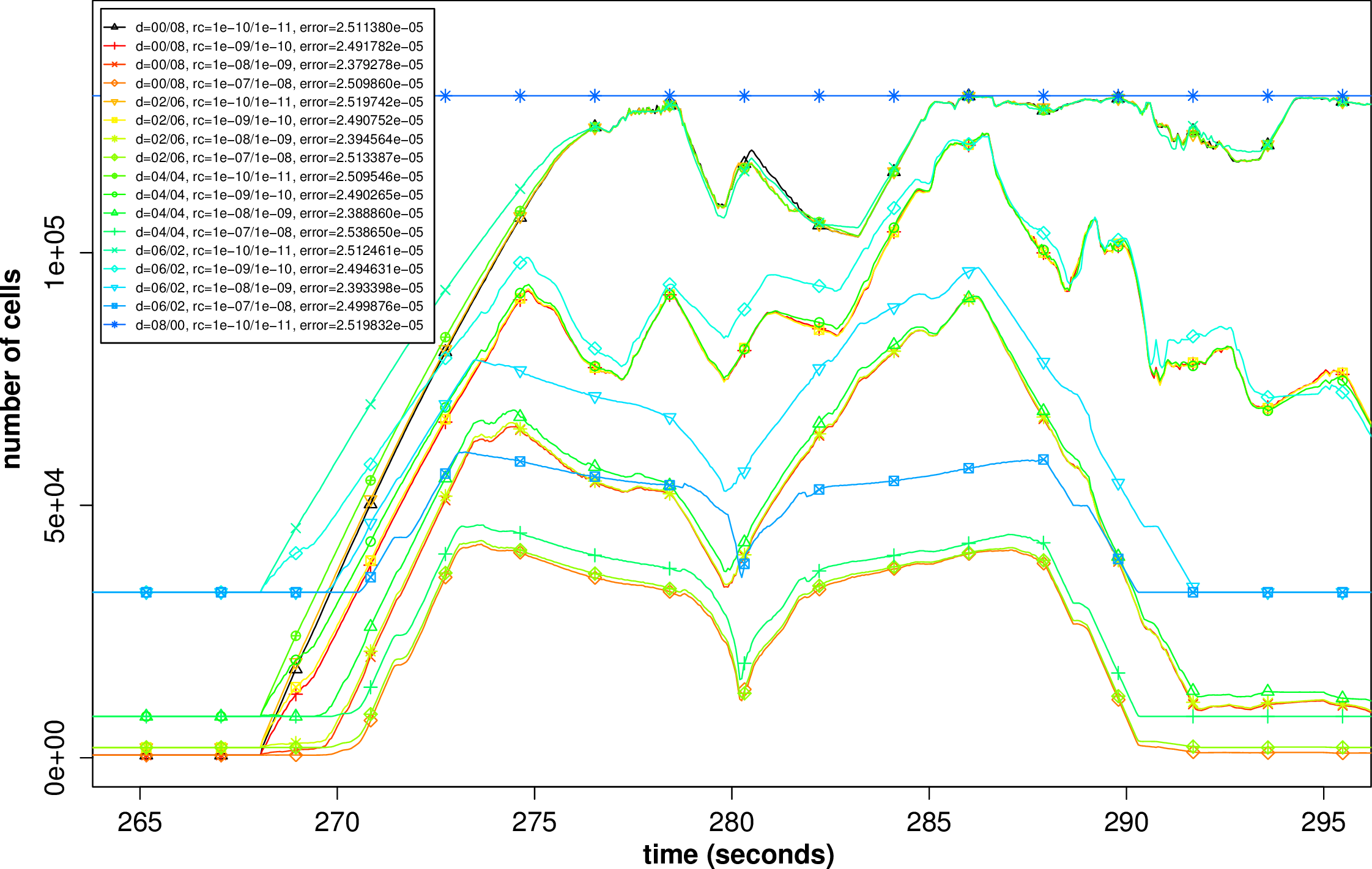
In the next step, we have a closer look on the parameter studies which do not only yield improved results, according to the L1 error norm, but also require less cells in average. We use d = [initialrefinementdepth]∕[dynamicadaptiverefinementlevels] to abbreviate the adaptivity parameters. A plot for the corresponding cell distributions is given in Fig. 6.6 and detailed information is presented in the next table:
| Benchmark parameter | error | avg. cells | time steps | saved cells per time step |
| d=0/8, r=0.0001/0.00001 | 2.38e-5 | 23556.13 | 38839 | 28.1% |
| d=0/8, r=0.001/0.0001 | 2.51e-5 | 11795.13 | 30009 | 64.0% |
| d=2/6, r=0.0001/0.00001 | 2.39e-5 | 24326.79 | 40303 | 25.8% |
| d=2/6, r=0.001/0.0001 | 2.51e-5 | 12924.97 | 31354 | 60.6% |
| d=4/4, r=0.0001/0.00001 | 2.39e-5 | 28169.67 | 43500 | 14.0% |
| d=4/4, r=0.001/0.0001 | 2.54e-5 | 18075.68 | 36732 | 44.8% |
| d=6/0 (baseline) | 3.80e-5 | 32768.00 | 37553 | 0.0% |
| d=8/0 (baseline 2) | 2.52e-5 | 131072.00 | 75105 | -300.0% |
We can see, that for the “d=0/8, r=0.001/0.0001” parameter settings this yields an
improvement of  ≈ 64% cells used in average per time step and on the other hand,
we get more accurate results. Also considering the total amount of cells involved in the
computations, the benefit is increased to
≈ 64% cells used in average per time step and on the other hand,
we get more accurate results. Also considering the total amount of cells involved in the
computations, the benefit is increased to  ≈ 71.2% for the considered
parameters.
≈ 71.2% for the considered
parameters.
With a domain regularly resolved with a refinement depth d = 8, the computed error is 2.52e–5
after 75105 time steps. We compare this to the parameter study “d=0/8, r=0.001/0.0001” which
yielded the best result for the same order of magnitude . This leads to  ≈ 96.4%
less cells involved in the computations.
≈ 96.4%
less cells involved in the computations.
These benefits are based on conservatively chosen adapvitiy parameters and on simulations on a relatively small domain. Hence, we expect more improvements by further parameter studies and larger domains. In the next chapter, we evaluate the potential of the dynamic adaptivity on a realistic Tsunami simulation.