These html pages are based on the
PhD thesis "Cluster-Based Parallelization of Simulations on Dynamically Adaptive Grids and Dynamic Resource Management" by Martin Schreiber.
There is also
more information and a PDF version available.
6.3 Field benchmark: Tohoku Tsunami simulation
With the simulation of the Tohoku Tsunami of 11 March 2011, a realistic benchmark is given to show
the potential of the developed algorithms for dynamically adaptive mesh refinement. Here, we assume
that the information on the water surface displacement information due to earthquakes is available a
short time after the earthquake.
Acknowledgements for the Tsunami simulation
The first dynamically adaptive Tsunami parameter studies with our cluster-based parallelization
approach were simulated in the beginning of 2012. These simulations were developed in collaboration
with Alexander Breuer who contributed, among others, the required C++-interfaces to
the GeoClaw Riemann solver, the bathymetry and displacement datasets. Also Sebastian
Rettenberger contributed his development ASAGI [Ret12] to this studies to access the bathymetry
datasets.
However, this was not used anymore for the studies in this thesis due to reasons discussed in the
following section. We also like to thank the Clawpack- and Tsunami-research groups for providing
their software and the scripts as Open Source and a very good documentation to reproduce their
results.
Bathymetry and multi-resolution sampling
Due to dynamic adaptivity, the bathymetry data has to be sampled during run time.
The bathymetry datasets we used in this work are based on the
GebCo
dataset with its highest resolution requiring 2GB of memory. With the different cell resolutions,
sampling the bathymetry dataset only on the finest level would lead to aliasing effects, and special
care has to be taken with interpolation [PHP02]. Therefore, we additionally preprocessed the
bathymetry computing multi-resolution bathymetry datasets. Using multiple resolutions, the coarser
levels then require  of memory compared to the next higher-resolved level, thus the overall memory
requirement is less than 3GB to store all levels. This memory requirement is considerably lower than
the total memory available per shared-memory compute node. Therefore, we decided to use a
native loader for the bathymetry data which loads the entire bathymetry datasets into the
memory.
of memory compared to the next higher-resolved level, thus the overall memory
requirement is less than 3GB to store all levels. This memory requirement is considerably lower than
the total memory available per shared-memory compute node. Therefore, we decided to use a
native loader for the bathymetry data which loads the entire bathymetry datasets into the
memory.
For the Tohoku Tsunami simulation, the GebCo dataset is preprocessed with the Generic Mapping
Tools [WS91]; they map the bathymetry data given in longitude-latitude format to the area of
interest, see Fig. 6.7. We used a length-preserving mapping, which conserves the length from each
point on the bathymetry data to the center of the displacement data.
Initialization
For the Tohoku Tsunami, an earthquake resulted in displacements of the sea ground which led
to a change of the water surface height. We consider a model which assumes a change
in the water surface only at the beginning of the simulation. Hence, for the initial
time step of the Tsunami simulation, we require the information on the displacements
describing these surface elevation and follow the instructions provided within the Clawpack
package . The seismic data we
use is provided by the UCSB
and used as input to the Okada model [SLJM11] computing the displacements.
Our initialization is based on an iterative loop:
-
(1)
- In each iteration, the conserved quantities are reset to the state at time t = 0.
These conserved quantities are the water surface height including the displacement. The
bathymetry data is sampled from the multi-resolution datasets, and both momentum
components are set to zero.
-
(2)
- Then, a single time step is computed and the grid is refined with adaptivity requests based
on the net-update parameters (see Sec. 6.1.3).
-
(3)
- If the grid structure changed, continue at (1), otherwise continue with the simulation.
This setup relies on the local extrema of the displacement datasets already detectable by the
net-update error indicator.
Adaptivity parameters
Similar to the analytic benchmark in Sec. 6.2, we conducted several benchmarks with different initial
refinement parameters d = {10,16,22} and up to a = {0,6,12} additional refinement levels. The
refinement thresholds used by the error indicators are r = {50,500,5000,50000} and c =  for the
coarsening thresholds.
for the
coarsening thresholds.
Comparison with buoy station data
We first conducted studies by comparing the smiulation data with the water-surface
elevation measured at particular buoy stations. This elevation data is provided by
NOAA .
The tidal waves are not modeled within our simulation, but included in the buoy station data.
To remove this tidal-wave induced water-surface displacement, we use the detide scripts
(see [BGLM11]).
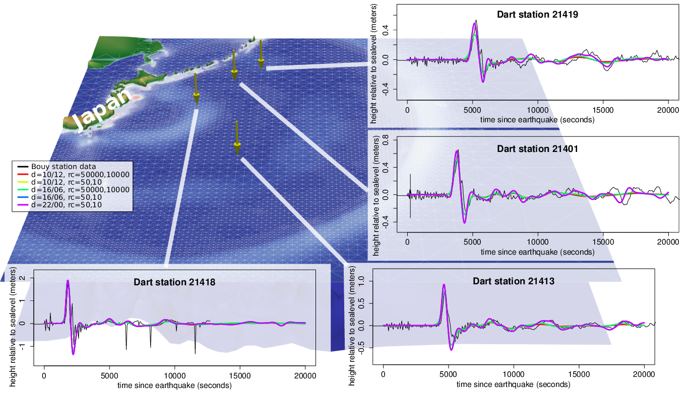
The simulation domain and the simulated and measured displacements of the buoy stations are
visualized in Fig. 6.7. This visualization of the simulation grid and the water and bathymetry data is
based on a simulation with adaptivity paramters chosen for a comprehensible visualization of the
grid.
Regarding the time of the wave front hitting the buoy station, the results show a very good
agreement with the data recorded by the buoy stations. However, we should consider that the
underlying simulation is based on displacement data computed with a model. Therefore, no concrete
statement in the direction of a realistic simulation should be made here, but we continue determining
the possibilities with our dynamically adaptive simulations.
Dynamically adaptive Tsunami simulations
We executed Tsunami simulations with the adaptivity parameters described in the previous section.
To reduce the amount of data involved in our data analysis, we selected a particular buoy station. We
expect, that wave propagations to buoy stations over a longer time are more influenced by factors such
as the grid resolution and other parameters compared to wave propagations which take only
a short time to reach a buoy station. Therefore we select buoy station 21419, with the
peak of the first wave front arriving at the latest point in time compared to the other
stations.
We compute the error norm (6.1.2) on the time interval [0,20000] for several adaptivity
parameters; the results are given in Table 6.1. Figure 6.8 shows bar plots of the errors and the
normalized average number of cells relative to the maximum value. Dynamically adaptive simulations
require an improvement in the error and the number of cells. Detailed results are discussed
next.
|
|
|
|
| Parameter study | L1 error | Processed mio. cells | Saved cells |
|
|
|
|
|
|
|
|
| da=22/0 | 0 | 88936.02 | -719.16% |
|
|
|
|
| da=20/0 (baseline) | 0.026121 | 10856.96 | 0% |
|
|
|
|
| da=18/0 r=50/10 | 0.0306024 | 1298.14 | 88.04% |
|
|
|
|
| da=16/6 r=50/10 | 0.0005550 | 51775.64 | -376.89% |
|
|
|
|
| da=16/6 r=500/100 | 0.0013608 | 36650.05 | -237.57% |
|
|
|
|
| da=16/6 r=5000/1000 | 0.0055551 | 7342.58 | 32.37% |
|
|
|
|
| da=16/6 r=50000/10000 | 0.0198121 | 1151.38 | 89.40% |
|
|
|
|
| da=16/0 | 0.0337187 | 150.34 | 98.62% |
|
|
|
|
| da=10/12 r=50/10 | 0.0005356 | 51275.72 | -372.28% |
|
|
|
|
| da=10/12 r=500/100 | 0.0013975 | 36127.60 | -232.76% |
|
|
|
|
| da=10/12 r=5000/1000 | 0.0055124 | 6784.04 | 37.51% |
|
|
|
|
| da=10/12 r=50000/10000 | 0.0213234 | 452.25 | 95.83% |
|
|
|
|
| da=10/6 r=50/10 | 0.0333180 | 97.43 | 99.10% |
|
|
|
|
| da=10/6 r=500/100 | 0.0333127 | 95.11 | 99.12% |
|
|
|
|
| da=10/6 r=5000/1000 | 0.0333143 | 75.89 | 99.30% |
|
|
|
|
| da=10/6 r=50000/10000 | 0.0325013 | 22.86 | 99.79% |
|
|
|
|
| da=10/0 | 0.0406040 | 0.26 | 100.00% |
|
|
|
|
| |
Table 6.1: Different parameter studies and computed error relative to the baseline da=22/0
and saved cells relative to the baseline da=20/0.
We use da = 20∕0 (initial refinement depth of 20, no additional refinement levels) as the
baseline for comparison with our dynamically adaptive grids. Comparing this baseline
with da = 22∕0 shows that about 8 times more cells are involved in the computation. This
is
-
(a)
- due to two additional refinement levels resulting in 4 times more cells and
-
(b)
- due to the reduced CFL condition.
With the computed error of 0.026121 for our baseline da = 20∕0, we first highlighted each computed error
with bold face and each number of processed cells below 10856.96 mio. in Table 6.1. Then, the
percentage of saved cells compared to the baseline is given in the right column. The last column shows
the possibilities with the impact of computational amount with our dynamic adaptivity: we can save
more than 95% of the cells required for yielding improved results according to the L1 error
norm.
We continue with a more detailed execution of the simulation on a Westmere 32-core
shared-memory system to determine the possible savings in computation time. The cluster split
threshold is automatically chosen, keeping the number of clusters close to 512. The regular resolution
created 512 clusters in average, yielding 16 clusters per core. We measure the time after the
initialization of the earthquake induced displacements. The timings for the simulation
traversals, adaptivity traversals and split/join phases are presented separately in the following
table:
|
|
|
|
| | Simulation parameters
|
|
|
|
|
| | da=10/12 r=50000/10000 | da=20/0 | da=22/0 |
|
|
|
|
|
|
|
|
| Simulation traversals | 13.63 sec | 288.09 sec | 2370.19 sec |
|
|
|
|
| Adaptivity traversals | 10.44 sec | 23.05 sec | 157.47 sec |
|
|
|
|
| Split/join operations | 7.84 sec | 5.41 sec | 11.22 sec |
|
|
|
|
|
|
|
|
| Sum | 43.71 sec | 336.03 sec | 2557.11 sec |
|
|
|
|
| |
The sum of all values is slightly different to the sum of all measured program phases due to, e.g.,
overheads induced by measurement. We can see, that the adaptivity traversals and the time spend
into the split/join operations exceed the time invested for the simulation traversals. However, this
relative overhead pays off due to the reduced overall computation time compared to the regular grid
resolution.
-
(a)
- da = 20∕0:
We start by comparing the simulation-traversal time for running the wave propagation
on the regularly resolved domain da = 20∕0 with the entire simulation time (time
stepping, adapvitity, split/joins) required by our dynamically adaptive simulation da =
10∕12,r = 50000∕10000. Compared to the simulation da = 22∕0, this yields a performance
improvement of  = 6.6.
We next analyze the theoretical maximum performance improvements based on the average
number of cells per time step: for the simulation on a dynamically adaptive grid, only 69070 cells
per time step are used in average whereas for the regular grid, 2097152 cells were processed
per time step, yielding a factor of 30.4 as the expected performance improvement.
However, we only gained a factor of 6.6 for which we account by the following three issues:
- The size of the dynamically adaptive grid with only 69070 cells in average per time
step is very small, resulting in a relatively low scalability.
- Additional overheads are introduced by the dynamically changing grid structure
- The number of required time steps is increased from 5177 for the da = 20∕0 simulation
to 6543 for the simulation on the dynamically adaptive grid. This is due to smaller
grid cells on the dynamically adaptive grid lead to a decreased time-step size.
-
(b)
- da = 22∕0:
Here, we assume that the simulation on the dynamically adaptive grids are sufficiently accurate so
that we can compare the refinement depth of the regularly resolved domain to the
maximum refinement depth of the dynamical adaptive simulation. This also avoids the
aforementioned issue (3) with smaller time steps. Then, we can compare the runtime of 43.71
seconds for the dynamically adapative simulation da = 10∕12,r = 50000∕10000 with the
simulation runtime of 2370.19 seconds for a regularly resolved domain da = 22∕0. Here, we
get a performance improvement of  = 54.2. To give another example for the
dynamically adaptive simulation with da = 10∕12,r = 10000∕2000, we still get a speedup of
= 54.2. To give another example for the
dynamically adaptive simulation with da = 10∕12,r = 10000∕2000, we still get a speedup of
 = 16.4. We want to emphazise again, that these speedups only hold under the
assumption, that the results of the dynamically adaptive simulation are sufficiently
accurate.
= 16.4. We want to emphazise again, that these speedups only hold under the
assumption, that the results of the dynamically adaptive simulation are sufficiently
accurate.
With simulations on dynamically changing grids, this also results in dynamically changing resource
requirements over the simulation runtime. E.g. considering the results for the dynamically adaptive
simulation in the aforementioned benchmark scenario (a), the simulation is not able to scale very well
on the assigned number of cores due to its small problem size. With concurrently executed
applications with dynamically changing resource requirements, e.g. multiple simulations
for parameter studies on dynamically adaptive grids, an over-runtime changing resource
assignment can result in increased efficiency on which we put our focus on in part IV of this
thesis.