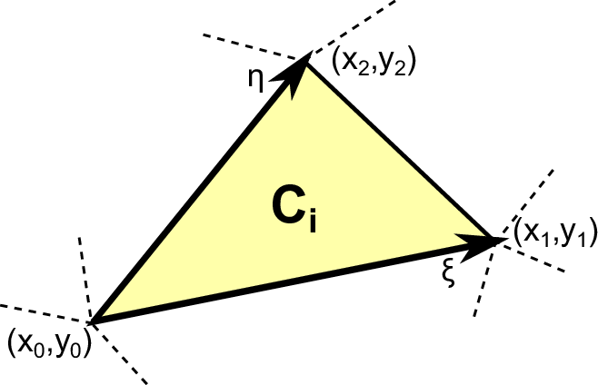
The entire simulation domain can be represented by a set of triangles

By applying affine transformations, each triangle Ci and the conserved quantities can be mapped from world space to a so-called reference triangle. For the sake of clarity, the formulae in the following sections are given relative to such a reference triangle.
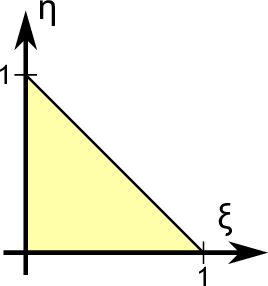
We use the triangle reference space with both triangle legs of a length of 1 and aligned at the x- and y-axes, see Fig. 2.3. The support in reference space is then given by
![T = {(ξ,η) ∈ [0,1]2 | ξ ≥ 0 ∧η ≥ 0 ∧ ξ + η ≤ 1}. (2.1)](schreiber14dissertation26x.png)
Using a homogeneous point representation, mappings of points from reference to world space are achieved with
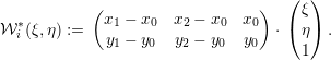
Assuming a mathematical formulation which is independent of the spatial position of the triangle, we can drop the orientation-related components and simplify this mapping to
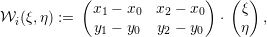
 | (2.2) |
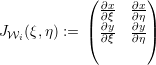
computing the derivatives in world space with respect to reference space coordinates (ξ,η). Affine transformations to and from world space can then be accomplished by additional projections of particular terms (see [AS98,HW08]) and for our simulations on the sphere in Section 6.5.
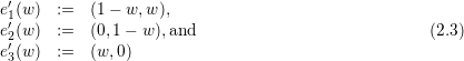
With the points
parameterized with w, the interval for each edge is given by ei := {e′i(w)|w ∈ [0,1]}. Note the unique anti-clockwise movements of the points e′i(w) for all edges and a growing parameter w which is important for the unique storage order of quantities at edges.For the remainder of this chapter, we stick to the world-space coordinates.