These html pages are based on the
PhD thesis "Cluster-Based Parallelization of Simulations on Dynamically Adaptive Grids and Dynamic Resource Management" by Martin Schreiber.
There is also
more information and a PDF version available.
2.7 Flux matrices 
The flux term ∮
dT (F(∑
iUi(t)φi(ξ,η))φj(ξ,η)) ⋅ (ξ,η) in Eq. (2.9) represents the change of
conserved quantities via a flux across an edge. With the non-overlapping support of any two
adjacent triangles, also the approximated solution is unsteady at the triangle boundaries.
By considering each triangle edge separately, we can evaluate the edge-flux term in three
steps:
(ξ,η) in Eq. (2.9) represents the change of
conserved quantities via a flux across an edge. With the non-overlapping support of any two
adjacent triangles, also the approximated solution is unsteady at the triangle boundaries.
By considering each triangle edge separately, we can evaluate the edge-flux term in three
steps:
-
1.
- First, we evaluate our approximated solution at particular quadrature points on the edge,
see left image in Fig. 2.4. Here, we can use a beneficial property of the GL quadrature
points (see Sec. 2.3.1): one-dimensional GL quadrature points on the edge directly coincide
with the GL quadrature and are thus nodal points of the reference triangle. Therefore,
computing the conserved quantities at the quadrature points only involves the conserved
quantities stored at these points. See Appendix A.1.5 for the sparse matrix selecting the
corresponding conserved quantities.
-
2.
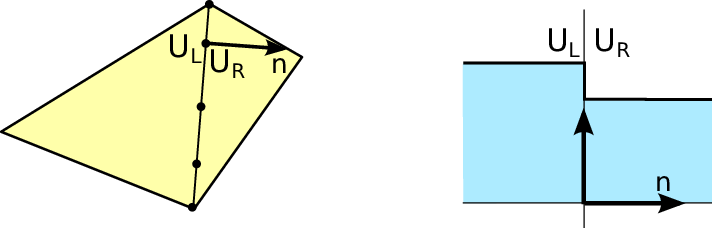
- Second, the flux is computed at the quadrature points based on pairs of selected
coinciding quadrature points from the local and the adjacent cell. We can simplify this
two-dimensional Riemann problem to a one-dimensional one (see right image in Fig. 2.4)
by changing the basis to the edge normal taken as the x-basis axis and the discontinuity
on the edge at x = 0: Only considering a single conserved quantity on an edge, ÛL and ÛR
represent the current solution Û on the left and right side of the y-axis, respectively. The
change over time can then be computed by using flux solvers which is further discussed
in Sec. 2.10.
-
3.
- Third, we reconstruct our approximated solution ∑
iF(Ui(t))φi(ξ,η) for each edge based
on the computed flux crossing the edge [GW08]. By splitting the surface integral ∮
dT over
the triangle reference boundaries into three separate integrals ∑
e∈E ∮
de over each edge
e ∈ E (see Section 2.2) and factoring out the term with the computed flux approximation
from the integral, this yields
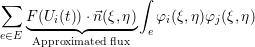 with the evaluation of the Riemann problem term F(Ui(t)) ⋅
 (ξ,η) further described in
Section 2.10. Note that the “Approximated flux” term may also depend on other conserved
quantities than Ui. Solutions for this integral can again be stored in matrices similarly
to the previous sections. For GL points, these matrices are again sparse and influence
conserved quantities only if these are stored on the corresponding triangle’s edge (see
Appendix A.1.5).
(ξ,η) further described in
Section 2.10. Note that the “Approximated flux” term may also depend on other conserved
quantities than Ui. Solutions for this integral can again be stored in matrices similarly
to the previous sections. For GL points, these matrices are again sparse and influence
conserved quantities only if these are stored on the corresponding triangle’s edge (see
Appendix A.1.5).
The presented method is a quadrature of the flux on each edge with fluxes evaluated at pairs of
given quadrature points. Rather than evaluating the flux for several pairs of given points, alternative
approaches use flux computations based on a single pair of given functions [AS98]. These functions
represent the conserved quantities on the entire edge. Since the interfaces derived in this framework
can be also used for such an implementation, we continue using the previously described method
without loss of applicability.