These html pages are based on the
PhD thesis "Cluster-Based Parallelization of Simulations on Dynamically Adaptive Grids and Dynamic Resource Management" by Martin Schreiber.
There is also
more information and a PDF version available.
A.1 Hyperbolic PDEs
A.1.1 Gauss Lobatto Points
The following table gives examples of basis functions based on Gauss-Lobatto points and their nodal
points up to order 2.
|
|
|
| | Polynomial | Nodal point |
|
|
|
| Degree 0: | φ0(x,y) := 1 | ( , , ) ) |
|
|
|
| Degree 1: | φ0(x,y) := 1 - x - y | ( , , ) ) |
| | φ1(x,y) := x | ( ,0) ,0) |
| | φ2(x,y) := y | (0, ) ) |
|
|
|
| Degree 2: | φ0(x,y) := 1 - 3x + 2x2 - 3y + 4xy + 2y2 | (0,0) |
| | φ1(x,y) := 4x - 4x2 - 4xy | ( ,0) ,0) |
| | φ2(x,y) := -x + 2x2 | (1,0) |
| | φ3(x,y) := 4y - 4xy - 4y2 | (0, ) ) |
| | φ4(x,y) := 4xy | ( , , ) ) |
| | φ5(x,y) := -y + 2y2 | (0,1) |
|
|
|
| |
A.1.2 Jacobi polynomials
The orthogonal Jacobi polynomials on triangle basis up to degree 2 are given in the following
Table. Compared to the Gauss-Lobatto Points, the Jacobi polynomials are constructed
hierarchically.
|
|
|
| | Polynomial |
|
|
|
| Degree 0: | φ0(x,y) :=  |
|
|
|
| Degree 1: | φ0(x,y) :=  |
| | φ1(x,y) := -2 + 6y |
| | φ2(x,y) := 2 (2x - 1 + y) (2x - 1 + y) |
|
|
|
| Degree 2: | φ0(x,y) :=  |
| | φ1(x,y) := -2 + 6y |
| | φ2(x,y) := (1 - 8y + 10y2) |
| | φ3(x,y) := 2 (2x - 1 + y) (2x - 1 + y) |
| | φ4(x,y) := 3 (-1 + 5y)(2x - 1 + y) (-1 + 5y)(2x - 1 + y) |
| | φ5(x,y) := (1 - 2y + y2 - 6x + 6xy + 6x2) |
|
|
|
| |
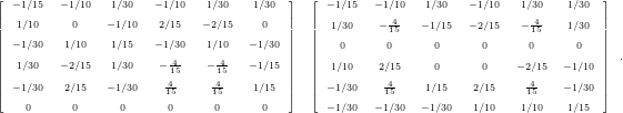
A.1.3 Mass Matrix
For nodal basis functions of degree 1 and 2 with Gauss-Lobatto points, the inverse mass matrices are
given by
Using orthonormal triangle basis functions based on normalized Jacobi Polynomials, the inverse mass
matrix is identical to the identity matrix for arbitrary degree.
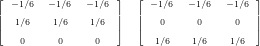
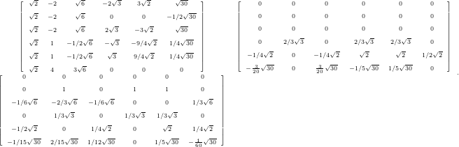
A.1.4 Stiffness matrices
For Gauss-Lobatto nodal points, this leads to stiffness matrices each with a single zero-row for degree
1:
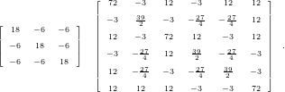
Computing the matrices x and y for degree 2, this still leads to almost dense matrices.
The matrices created for the orthonormal basis function have a higher sparsity pattern. Stiffness
matrices for degree 1 are given by
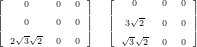
and for degree 2
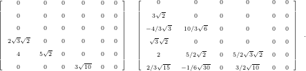
Those matrices have clearly a sparser layout and are thus better suited for computation considering
the stiffness matrices only so far.
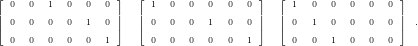
However, using modal basis functions, they have to be transferred to nodal basis functions. Using
Gauss-Lobatto nodal points and 1st degree basis functions, this results in the following three
matrices:
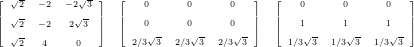
and to the following matrices for 2nd degree
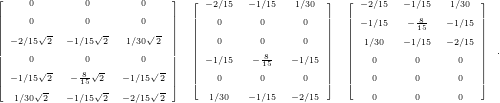
A.1.5 Flux matrices
Only a subset of conserved quantities is involved in the flux computation, see the following matrices
for GL nodal points of order 2:
 Thus each row selects the conserved quantities for each nodal point. For modal representation, a
similar approach to the stiffness matrices has to be used.
Thus each row selects the conserved quantities for each nodal point. For modal representation, a
similar approach to the stiffness matrices has to be used.
After flux computations, the flux updates only involve the nodal points of the edge for which
the flux was computed for. Examples for such matrices generated for flux computations
and Gauss Lobatto nodal points in the order of hypotenuse, right and left edge are given
by
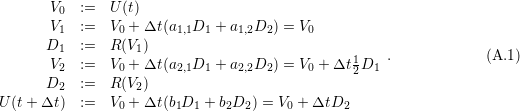
A.1.6 Butcher tableau
For RK with 2 stages, one possible tableau is
|
|
| a1,1 := 0 | a1,2 := 0 |
|
|
a2,1 :=  | a2,2 := 0 |
|
|
|
|
| b
1 := 0 | b2 := 1 |
|
|
| |
yielding
Another formulation for 2nd order accuracy is given by Heun’s method, yielding the tableau
|
|
| a1,1 := 0 | a1,2 := 0 |
|
|
| a2,1 := 1 | a2,2 := 0 |
|
|
|
|
b1 :=  | b2 :=  |
|
|
| |
The tableau for RK3 [But64] yielding 3-rd order accuracy is given by
The tableau for classical RK4 yielding 4-th order accuracy [SM03] is given by
|
|
|
|
| a1,1 := 0 | a1,2 := 0 | a1,3 := 0 | a1,4 := 0 |
|
|
|
|
a2,1 :=  | a2,2 := 0 | a2,3 := 0 | a2,4 := 0 |
|
|
|
|
| a3,1 := 0 | a3,2 :=  | a3,3 := 0 | a3,4 := 0 |
|
|
|
|
| a4,1 := 0 | a4,2 := 0 | a4,3 := 1 | a4,4 := 0 |
|
|
|
|
|
|
|
|
b1 :=  | b2 :=  | b3 :=  | b4 :=  |
|
|
|
|
| |
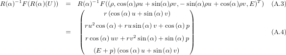
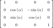
A.1.7 Rotational invariance of Euler equations
Here, we present the rotational invariancy of the Euler equations [Tor01]: For an edge normal  e
pointing towards (cos(α),sin(α))T , the rotation matrix R(α)e is given by
e
pointing towards (cos(α),sin(α))T , the rotation matrix R(α)e is given by
We test for rotational invariancy by putting the flux terms from Eq. (1.9) into the rotational
invariancy formula given in Eq. 2.9 which yields for the left hand side
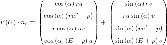 | (A.2) |
and for the right hand side
which is equal to F(U) ⋅ e using basic trigonometric calculus.