Parallelization with clusters

These html pages are based on the PhD thesis "Cluster-Based Parallelization of Simulations on Dynamically Adaptive Grids and Dynamic Resource Management" by Martin Schreiber.
There is also more information and a PDF version available.

[next] [prev] [prev-tail] [tail] [up]

5.3 Parallelization with clusters

Based on the previous sections which gave a description on our domain decomposition approach and the communication between partitions, we now describe implementation details of our parallelization approach: how to store and manage partitions. This finally leads to an efficient clustering of the grid as suggested in different contexts such as cluster-based local time stepping [CKT09] and clustering based on intervals of one-dimensional representations of SFCs preserving the locality of multi-dimensional grid traversals [MJFS01]. With our dynamic adaptive grid, we extend these ideas to a dynamic clustering.

5.3.1 Cluster definition

We start with our definition of a cluster by its data storage, grid management, communication meta information and traversal meta information properties:

Bulk of connected cell data:
In general, a bulk of cells connected via hyperfaces is associated uniquely to a cluster. There is a path from each cell to all other cells inside the cluster via shared hyperfaces of cells in the cluster. Using a continuous SFC, the connectivity is directly given by our partitioning approach based on SFC intervals and Theorem 4.3.1.
Indepent memory areas:
The simulation data and the meta information associated to each cluster is allocated in a way to be race-condition free with other clusters. In this work, we allocate the data for each cluster on a separate heap memory. Among others, this allows shrinking and growing of the number of grid cells in each cluster without forcing reallocations of data areas of other clusters.
Communication information:
The inter-partition communication should be managed efficiently for shared- and distributed-memory parallelization. In our case, we store such communication meta information to adjacent clusters using RLE. For the intra-partition communication, we use the stack-based communication approach. Communicating via stacks makes our communication invariant to the memory or rank location of the cluster, which becomes an important property for data migration.
Traversal meta information and user-specified data (optional):
Each cluster also has to store traversal meta data, e.g. initial vertex coordinates to start the grid traversal, minimum and maximum adaptive refinement depth limiters and also possibly required user-specified data. The traversal meta data is required to know where to start traversals in the spacetree. The user-specified data can consist of e.g. parameters for kernels and the face identifier of the cubed sphere, see Sec. 6.5.

pict

Figure 5.8: Examples of alternative clustering strategy: Shapes of clusters used for cluster-based local time-stepping method [CKT09]. The connectivity information is given via the edges shared by adjacent clusters. Such clusters are not generated by the approach presented in this thesis.

For cluster-based local time stepping [CKT09], a decomposition of the domain in non-overlapping bulks with communication schemes capable of independent time steps was suggested, see Fig. 5.8. Since our development yields the same possibilities with a domain decomposition based on the heuristic of the Sierpiński SFC, we continue to use the terminology cluster, referring to a partitioning and software design fulfilling the previously mentioned properties.

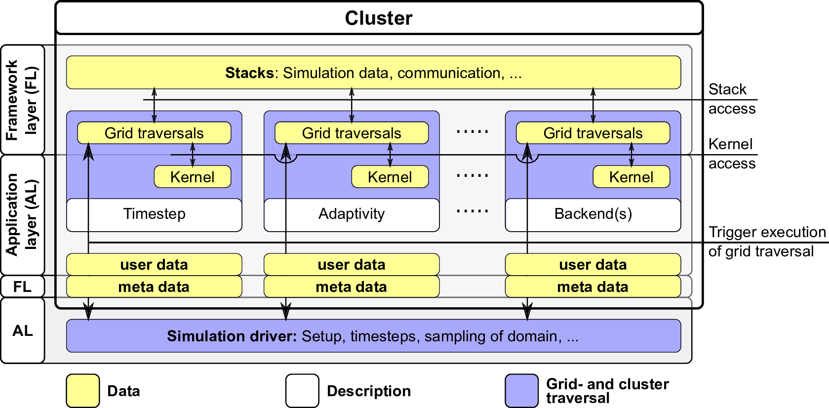
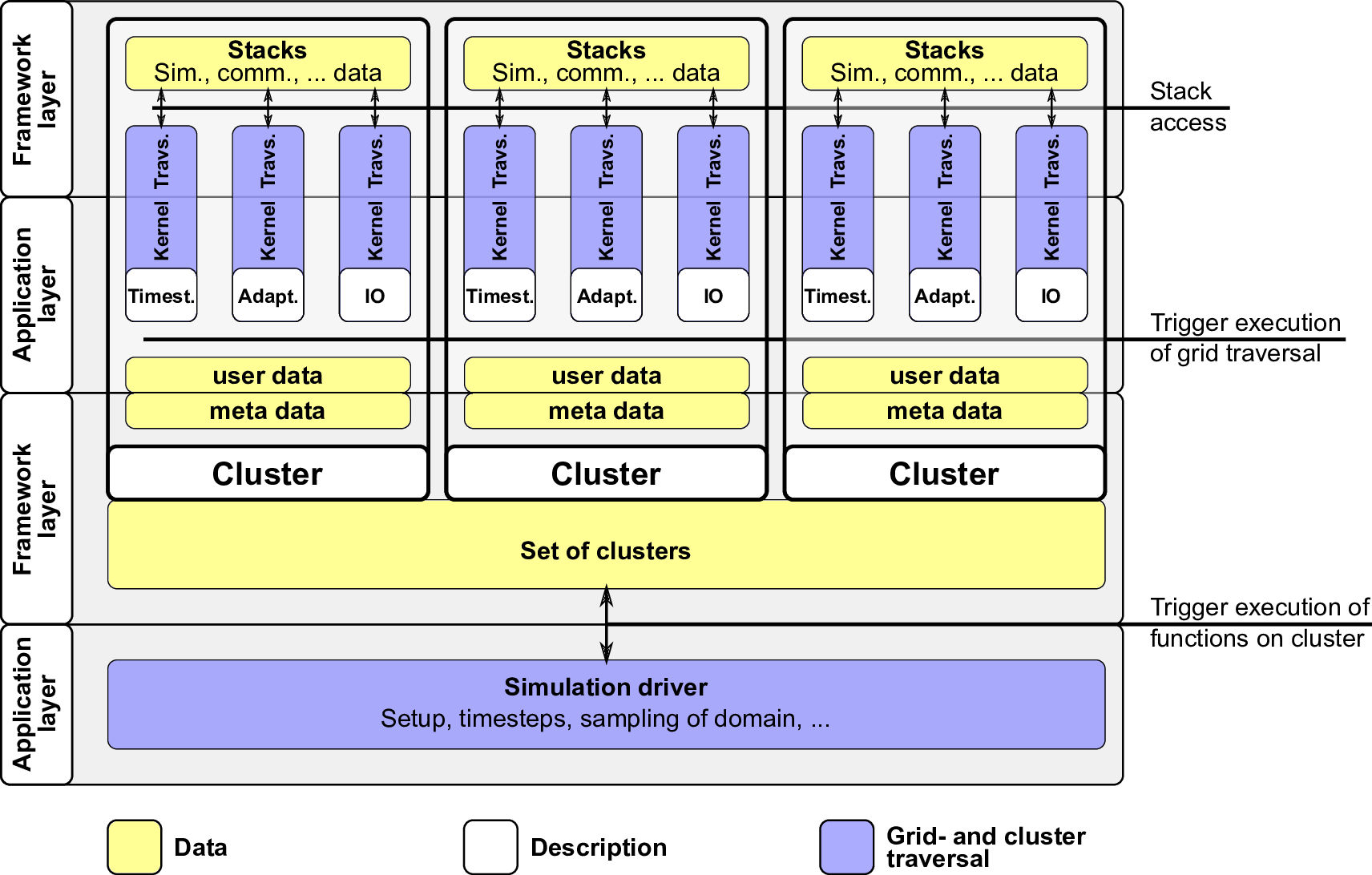
5.3.2 Cluster-based framework design

With clustering at hand, we introduce a parallel framework design with a top-down approach by assembling domains with a set of clusters: First, we encircle the simulation data, the grid traversals as well as the corresponding kernels from the serial framework design (see Fig. 4.12) into a cluster container. A sketch of the resulting structures and abstractions inside such a container are depicted in Fig. 5.9.

pict

Figure 5.9: Cluster building block based on serial framework design.

pict

Figure 5.10: Overview of the parallel cluster-based framework design. See the text for a detailed description.

For multiple clusters, we then extend this serial cluster-based framework design as it is depicted in Fig. 5.10. We continue with a top-down description under consideration of the serial framework design from Fig. 4.12:

Top framework layer: each cluster has associated its own grid data which is stored on stacks.
On the application layer below, kernels can be executed in parallel for each cluster without influencing each other due to replicated data scheme. The user data can be used to store cluster-specific information, e.g. the face id for the cubed-sphere domain triangulation or cluster-specific boundary conditions.
The meta data is required for communication and information on grid traversals and hence belongs to the framework layer. All clusters are kept in an efficient cluster management structure, the set of clusters, which is discussed in Section 5.3.3.
The simulation driver then executes operations specified via C++ lambda functions. These lambda functions are executed on all clusters with the cluster as the parameter. Such an operation in a lambda function can be e.g. a forward traversal or setting the cluster parameters.

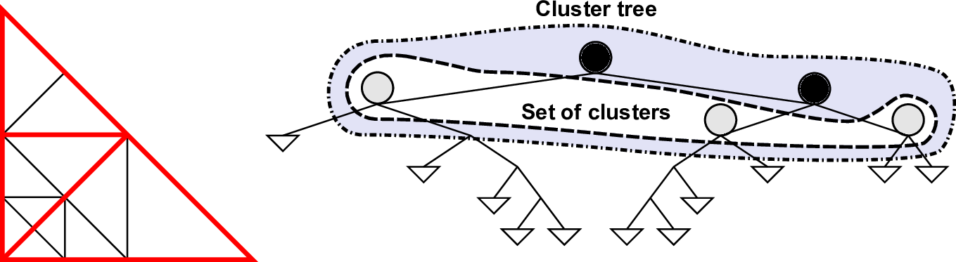
5.3.3 Cluster set

The dynamical creation and deletion of clusters demands for an efficient cluster management data structure. Such an efficient management can be e.g. achieved with (double-)linked lists, vectors and maps. All these containers represent a set which stores the clusters. With our dynamic cluster generation based on subtree, we keep the recursive structure and use a binary tree structure, the cluster tree, to insert and remove clusters.

In case of a cluster split, two nodes are attached to the formerly leaf node and the cluster data is initialized at both leaf nodes.

For clusters stored at two leaves sharing the same parent, a join operation creates new cluster data at the parent node. Here, we can also reuse the cluster storage of one children to avoid copy operations. After joining two clusters, both leaf nodes are removed.

See Section 5.5 for a detailed description of dynamic clustering. An example of a cluster set based on a tree is given in Fig. 5.11.

pict

Figure 5.11: Set of clusters based on tree-splits of the spacetree.

Regarding the base triangulation which allows us to assemble domains with triangles being their building blocks (see Section 5.4), we follow the idea from p4est [BWG11] and combine multiple cluster trees at the leaf of a super-cluster tree. This extends the cluster tree to a forest of trees, a cluster forest, embedded into the super-cluster tree. We avoid joining clusters which were not created by a cluster split, i.e. initially belonging to the base triangulation. Here, we limit the cluster-join operations by considering the depth of the cluster in the super-cluster tree. For sake of convenience, we continue referring to the super-cluster tree as the cluster tree.

5.3.4 Cluster unique ids

For identifying each cluster uniquely, we generate unique ids directly associated to the cluster’s placement in the cluster tree. This is based on the parent’s unique id for a split operation and childrens’ unique ids for join operation.

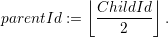
The cluster tree root id is initially set to 1_b with the subscript b denoting binary number notation. With the id of the parent node stored in parentId, the first child’s id traversed by the SFC and the second child’s id following the first child is given by

f irstChildId := 2⋅parentId and secondChildId := 2 ⋅parentId + 1.

Using this unique id inference results in a cluster forest’s root node id of 1_b - otherwise the same id would be assigned to the first child. Based on one of the child ids, the parent’s unique id can be inferred by

⌊ ⌋ parentId := ChildId- . 2

This recursive unique id generation also provides information on the placement of the cluster within the tree. This feature is used for cluster-based data migration in Section 5.10.3 to update adjacency information about cluster stored on the same MPI node.

Furthermore these unique ids inherently yield an order of the cluster along the SFC. Given id₁ and id₂, we can compute the order with the following algorithm: for each unique id, the depth of the cluster in the cluster tree is given with

clusterDepthi := bsr(idi)

(bit scan reversed), returning the position of the most significant set bit in id_i. E.g. bsr(001001₂) would yield 3. With the maximum depth of both clusters given by

maxClusterDepth := max (clusterDepth1, clusterDepth2),

we shift both unique ids to be on the same cluster tree level using

sidi := idi << (maxClusterDepth - clusterDepthi )

and finally get the order by direct comparison of both sid_i using less-than relations on sid_i represented with integer numbers. We can use this order to avoid duplicated reduce operations on replicated data shared by two clusters (see Section 5.8.1).

Alternative approaches would be e.g. based on a mix of MPI ranks and the MPI-node-local cluster enumeration. This also leads to properties which can be similarly used in the next sections. However, we decided to use the approach described above, since this unique id gets beneficial if searching for a cluster in the cluster tree.

[next] [prev] [prev-tail] [front] [up]