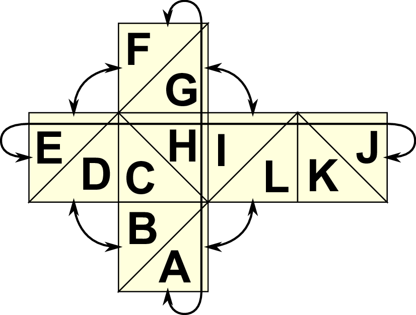
Figure 6.11: Cubed sphere domain triangulation with periodic boundary conditions.
Here, we present the possibility of simulations on the sphere based on our development. Using a two-dimensional quadrilateral domain shape and mapping this domain onto a sphere would lead to so-called pole singularities with sharp angles. Several solutions are available such as an icosahedral, a cubed sphere and a ying-yang grid (see [Beh06]). In this work, we use the cubed sphere, which was originally intended to be used for quadrilateral-like primitives.
With our framework being optimized for triangular grids created with a bisection, we start by assembling two triangles to a quadrilateral. Then each quadrilateral can be used as a cube face. This cube can be unfolded to a two-dimensional mesh which assembles the faces of a cube with a base triangulation given in Fig. 6.11. This figure also shows the cube-periodic boundary conditions with the arrows.
The cube’s center is assumed to be placed into the sphere’s center with a grid on each side of the cube. Then, each cube side is projected to the surface of the sphere and, due to the changes in angles, creates a distorted grid. Projection methods can then be e.g. equidistant or equiangular ones [NTL05].
To account for such a distortion of grid cells, the terms of our weak formulation of the continuity equation (see Eq. (2.8)) need to be extended to account for the projection of the cell from “sphere space” to “reference space”, see [Gir06] for detailed information. To compute these distortions, we require the knowledge on the cube’s face as well as the vertex coordinates on the sphere. Based on the two-dimensional vertex coordinates, we can then
Further extensions such as the Coriolis force and also the verification of the implementation of these projections is work under progress.
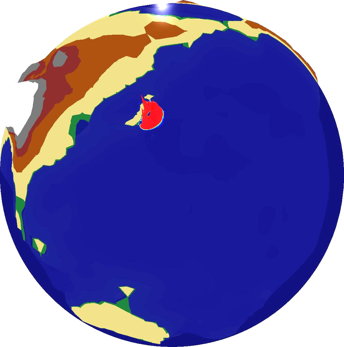
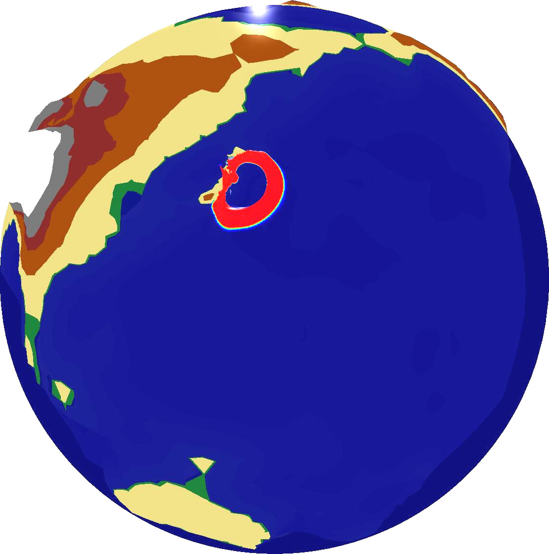
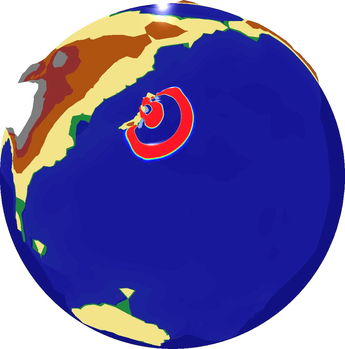
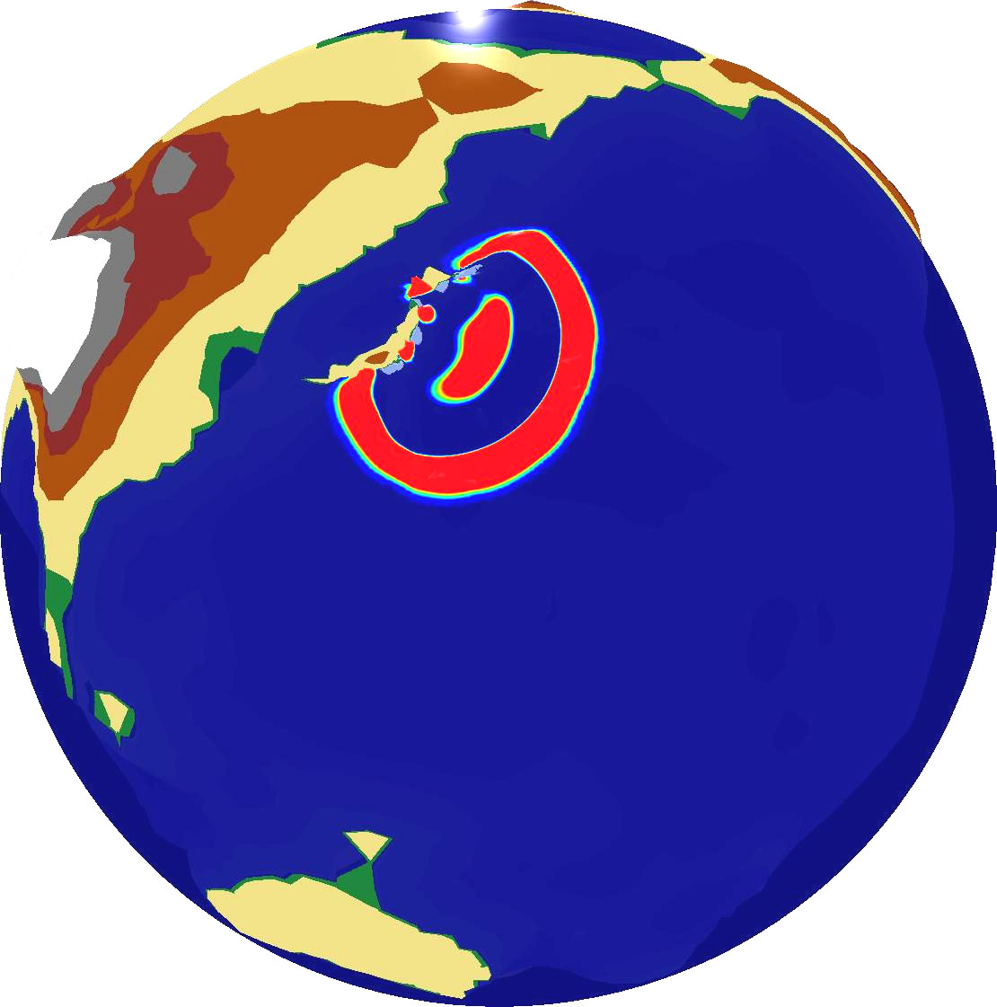
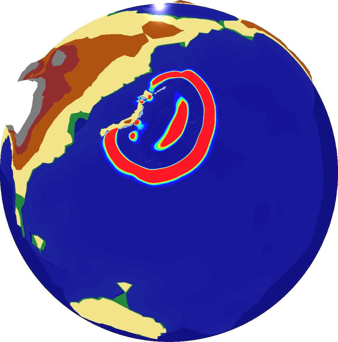
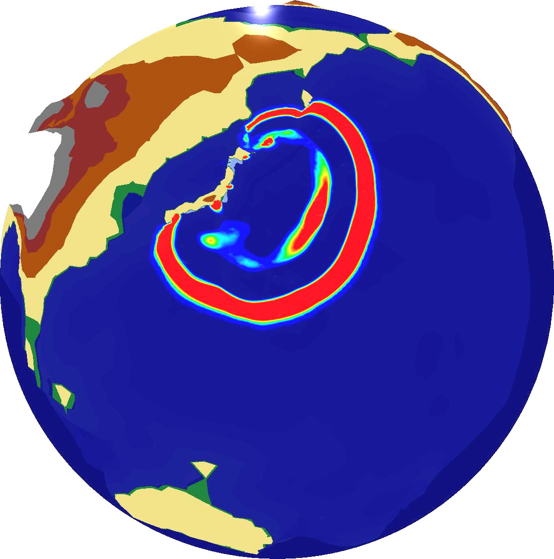
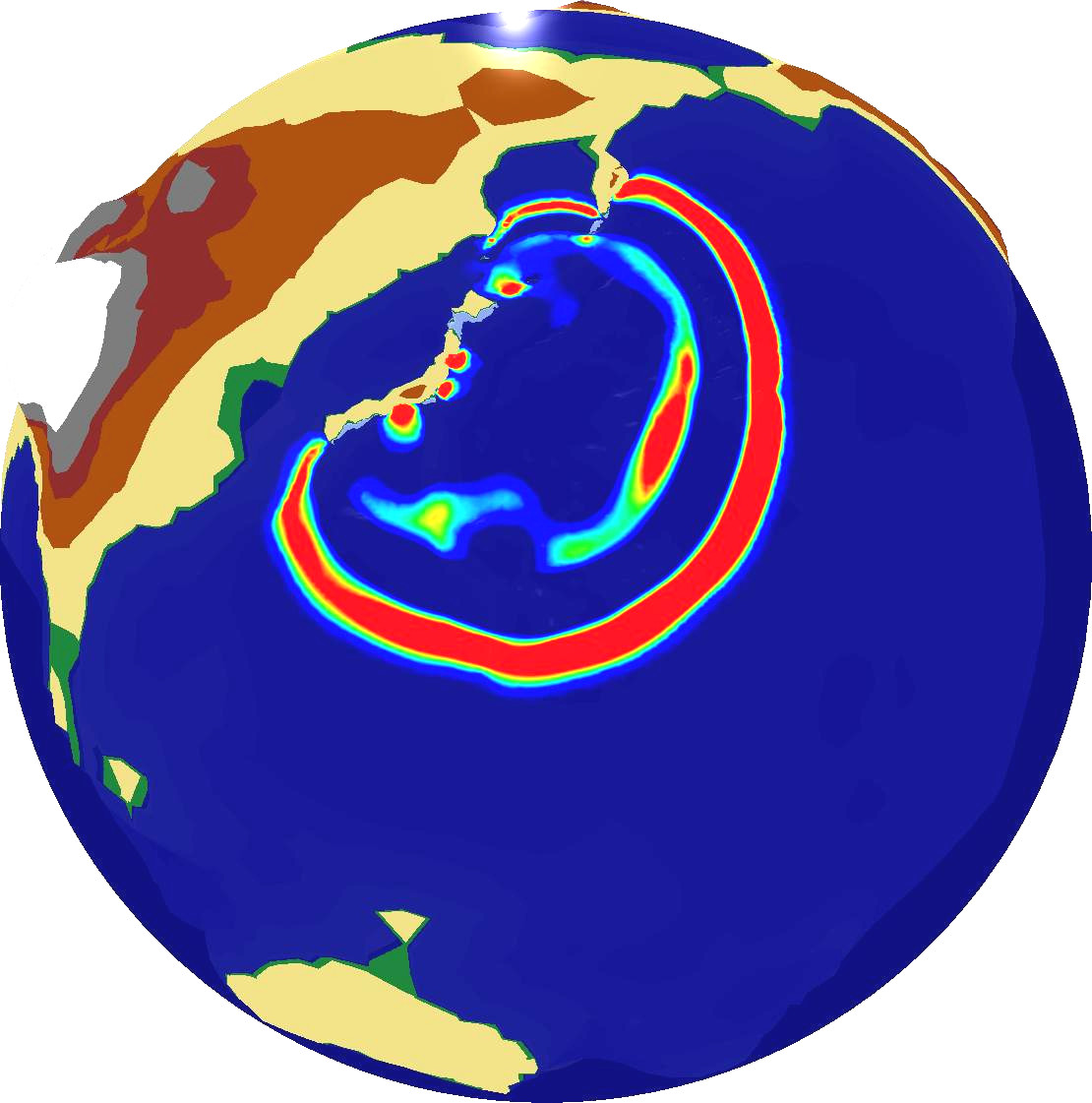
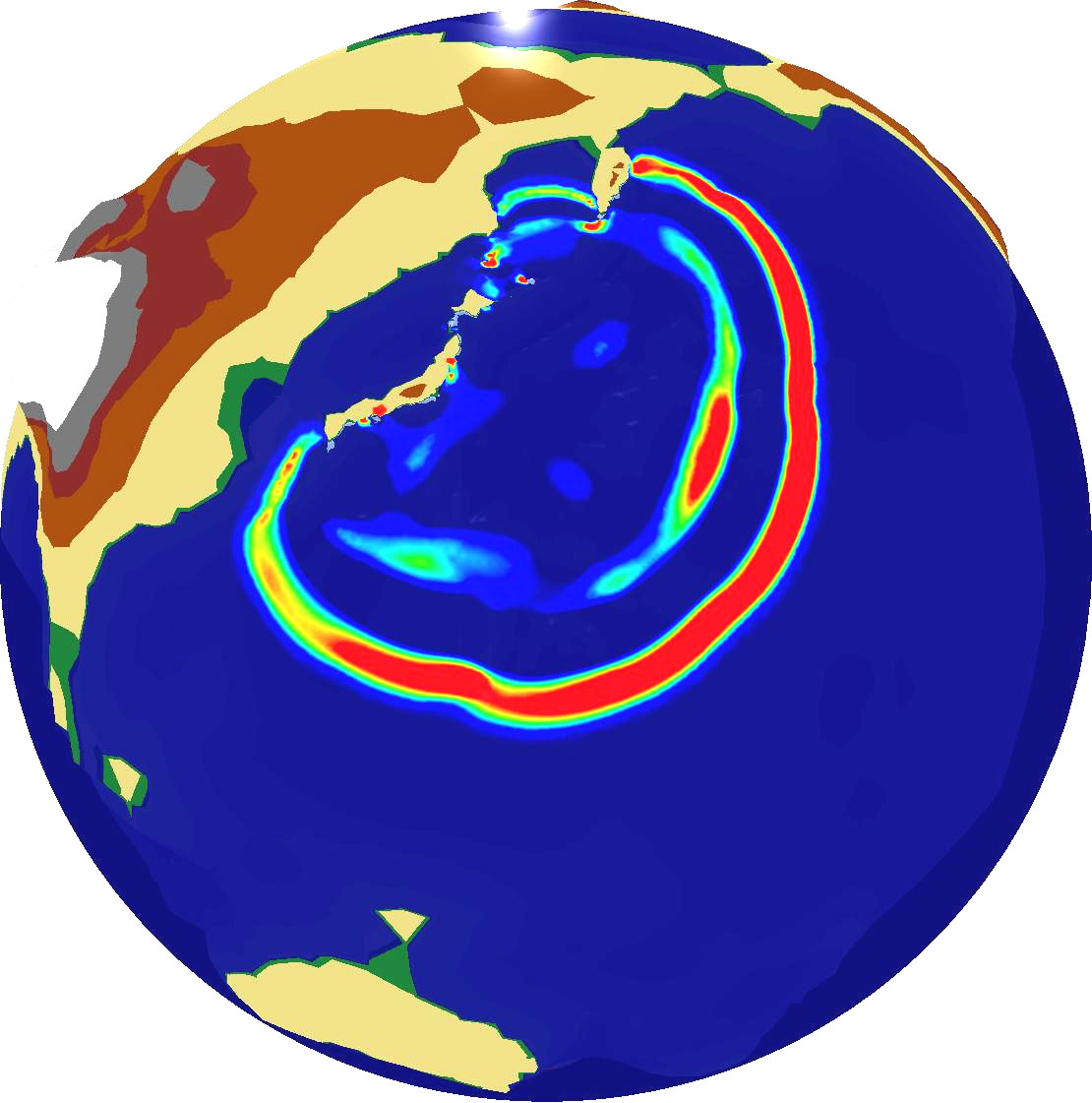
Combining this simulation with our OpenGL output backend which was discussed in Section 6.4.2, we can compute and directly visualize the propagation of the Tohoku Tsuami simulation over the entire earth globe based on the augmented Riemann solvers [Geo08]. Examplanory screenshots are given in Fig. 6.12.