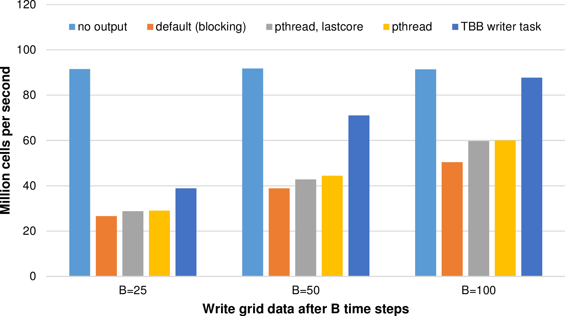
Figure 6.9: Benchmark statistics with million cells per second processed and for different output
backends. The parameter B specifies the number of time steps when to write data to persistent
memory.
The presented application scenarios are mainly driven to gain some insight into the simulated scenario. A visualization of the entire or a fraction of simulation data is one of the most frequently used way to gain this insight and we present different visualization backends.
We aim at generality of our backend infrastructure by considering both on- and off-line backends. For our off-line backend, we use VTK binary file output for off-line visualization with Paraview. Our on-line backend is based on OpenGL and also offers interactive steering of the simulation. The greatest common divisor for OpenGL and VTK backends regarding their simulation data storage format is storing of geometry and primitive data in separated arrays which we use as the input-data format to both backends.
Our main goals are then given by
With the interest of scientists to analyze the simulation data at different time steps, this data has to be made available for further processing. Using the VTK file backend, the data has to be written to persistent memory. However, typically only a very low bandwidth is available to access such a persistent memory compared to the main memory. Hence, also writing large datasets to it would result in severe bottlenecks and thus idling cores. Here, we studied several implementations to write the output data to persistent memory:
Using a writer task, other tasks can be processed by the same thread, e.g. with work stealing, after the task finished writing data to persistent memory.
The domain triangulation is based on a quadrilateral and the simulation grid is initialized with d = 10 and with up to a = 16 additional refinement levels. The simulation computes a radial dam break with the Rusanov flux solvers for 201 time steps. The output data itself is preprocessed in parallel by using all available cores. Such a simulation results in 4.55 mio. cells processed in average per simulation time step and with binary VTK file sizes above 300 MB. We used our Intel platform (see appendix A.2) and write the simulation output data to persistent memory (Western Digital Hard Drive of the typ Red 2 TB with a 64 MB cache and a theoretical transfer rate of up to 6 Gb/s). Results for different frequencies of writing output files to persistent memory are given in Fig. 6.9.
The blocking version shows a clear disadvantage compared to the other methods since cores idle until the function which writes the output data finished writing the data. Such idling cores are compensated with the pthread versions. Both pthread versions show an improvement. However, the dedicated writer core which we implemented to avoid oversubscription of cores leads to decreased performance of 0.85%, 3.68% and 0.42% percent respectively for writing output files each B = (25,50,100) time steps. Hence, avoiding resource conflicts does not result in a robust performance improvements for the tested simulation parameters. Here, the oversubscription of cores should be used.
With TBB fire-and-forget tasks, we get a robust performance improvement compared to all other writer methods. Furthermore, for writing the simulation data only after more than 100 time steps, the performance loss for writing data to persistent memory is only at 4% compared to writing no simulation data.
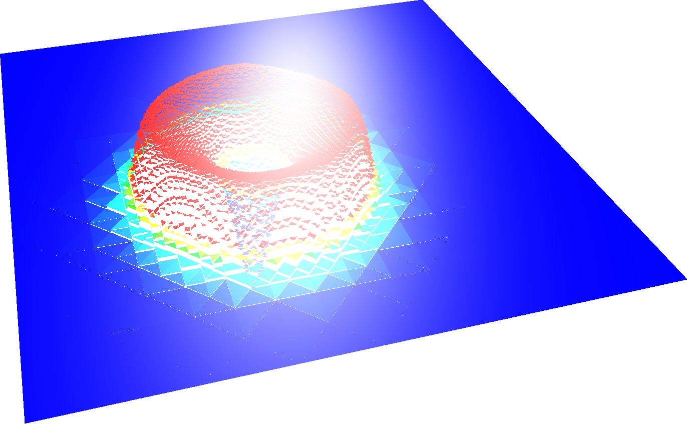
Besides the interactive steering possibilities of our OpenGL backend, here we like to focus on the reconstruction of a closed surface for visualization with the OpenGL backend with the vertex-based communication which was originally developed for node-based flux limiters. For shallow-water simulations, a direct visualization of the approximated solution with simulations based on the DG method leads to a surface with gaps. An examplanory visualization of a particular time step for a radial dam break is given in Fig. 6.10. Such gaps lead to a distraction of the person analyzing the data. For the visualization of a closed surface for shallow water DG simulations, cell data such as the water surface height can be averaged based on the surface height in cells sharing the vertex.
A generation of triangle strips for visualization was already considered with algorithms based on the Sierpiński SFC [PG07]. To our best knowledge, no visualization was developed so far which is capable of computing both vertex and normal data on-the-fly for surface reconstruction with dynamically adaptive triangular grids based on simulation data with a close to O(#cells) complexity.
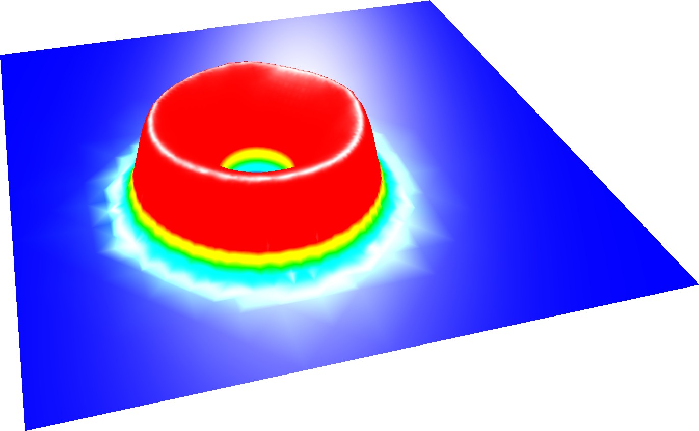
We compute a closed surface with our vertex-based communication scheme. Here, the per-cell approximated height is averaged at the vertices and used as the vertex for the water surface visualization. However, only considering vertex coordinates with a vertical displacement, e.g. based on water surface displacement, would not result in proper shading since normals are required at vertices. Therefore, we continue with additional traversals computing the normals associated to the previously computed vertices. This is based on the face orientations and quantitative properties for each triangle, see [JLW05] for further information.
Since traversing the cells is O(n) with a negligible overhead ϵ for reduce operations for a large cluster, and by using a fixed number of grid traversals, this also yields an O(n + ϵ) complexity for the reconstruction of our closed surface including the normals at each vertex. Other algorithms to reconstruct a closed surface such as the Voroni triangulation require at least an O(nlog n) algorithm in the worst-case [AK00], whereas our SFC traversal yields a robust O(n + ϵ) algorithm for the surface reconstruction, including cluster-based parallel processing.
Examples of the resulting surface visualization with the OpenGL backend are e.g. given in Fig. 6.10 and Fig. 6.12.