Figure 5.13: Backward traversal generating split information. The stacks generation direction
are given in forward traversal direction while the traversal itself is done in reversed direction
during the last backward adaptivity traversal [SBB12].
For our clusters based on tree splits, we use tree-split and -join operations for the cluster generation.
To split a cluster, we require information on (a) the number of shared hyperfaces along the separating hyperfaces and (b) the association of persistent data to both child clusters.
We achieve inferring this information by stopping our grid traversal at particular positions and implicitly derive the required quantities on the number of hyperfaces and cells based on the communication stacks (meta communication information) and persistent data stack (simulation data). We refer to this information as split information.
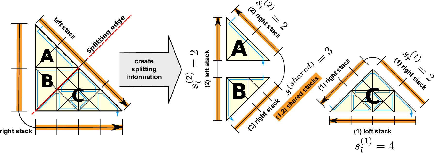
For optimization reasons, we can further join the determination of split information with the last backward adaptivity traversal and present the algorithm based on this backward traversal which is in reversed direction, see Fig. 5.13. The algorithm is based on the spacetree nodes on the 2nd level relative to the cluster root tree node and follows the SFC in reversed direction with (a,b,c,d). Here, we consider partitions (A,B,C) respectively set up by leaf nodes of subtrees (a,b,c ∪ d).
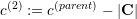
The application of our algorithm is given in Fig. 5.13 with the left and right communication stacks terminology used for the last adaptivity (backward) traversal and for grammars of type even. We denote the stacks for the left and right adaptivity communication stack with Sleft and Sright, respectively. The cell stack is given by C, and we determine the number of cells of the parent element by considering the elements stored on the cell stack: c(parent) := |C|.
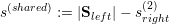
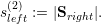
The information on the split operation is stored in s{left,right}(1) for the first and in s{left,right}(2) for the second child. We also require the number of edges shared by both split clusters in s(shared). The number of cells associated to the first and second child partition is stored to c(1) and c(2).


Clusters with leaf elements stored on level 1 or 2 require to be handled appropriately in case that subclusters A and B do not exist. E.g. with a domain only consisting of two cells, we can directly set sright(2) := 1, sleft(2) := 1, s(shared) := 1.
With the derived information, we can apply the split operation: The cell data on the stack can be directly split based on the split information c({1,2}). The traversal meta information (providing e.g. the starting point of the grid traversal) has to be updated to account for the new traversal start. The communication meta information of both children can also be determined, based on the information on the number of shared edges of both children given in s{left,right}({1,2}), s(shared) and c({1,2}). For the odd grid grammar, the inference of the required information is similar and therefore not further discussed here.
The presented algorithm only accounts for updating the local cluster information and would lead to inconsistencies to the meta information stored at adjacent cluster. Updating this meta information on adjacent cluster is presented in Section 5.5.3.
The simulation data on the stacks is currently split after the traversal of the entire cluster. However, copying chunks of stack data from the other clusters can result in stream-like copy operations and result in a bandwidth-limited problem. A direct streaming of the persistent simulation data during the last adaptivity traversal to the stacks of the corresponding new child clusters has the potential to avoid this additionally required stream-copy operation but is not implemented, yet.
Using clustering based on tree splits, our cluster-based approach is restricted to joining two clusters only if they share the same parent node in the cluster tree. Joining two clusters is accomplished by
So far, we can split and join clusters and update the meta information based on adaptivity markers written to the edge communication stacks. However, we also have to consider possible split and joins of adjacent clusters, e.g. if an RLE element has to be split to account for the associated cluster being split. This requires updating the edge communication meta information. We present an algorithm by modifying this edge communication information to synchronize with the adjacent meta communication information in case of splits or joins. This algorithm is based on local cluster and directly adjacent cluster access only and does not involve any global communication operations.
We continue refering to the cluster for which the RLE communication meta information is updated as the local cluster and a cluster described by a single RLE communication data stored for a local cluster as an adjacent cluster.
| Transfer State | Description |
| NO_TRANSFER | No split or join was executed on this cluster. |
| SPLIT_PARENT | This node was split and both children have the state SPLIT_CHILD. |
| SPLIT_CHILD | Cluster generated by a split operation are set to this state. |
| JOINED_PARENT | This node was created by joining both children which have state JOINED_CHILD. |
| JOINED_CHILD | This cluster represents a former child node which was joined with its sibling. This cluster is not deleted to allow accessing its communication meta information. |
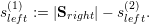
Updating edge-based meta communication is based on flags stored per cluster which describe the split- and join-states of the cluster. All required states for markers of adjacent clusters are given in Table 5.1 and an overview of all relevant cases which have to be considered in Fig. 5.14.
Similar to the exchange of edge communication data, updating the communication information is accomplished by read-only access of adjacent cluster data for shared memory access. Examples for the split-split constellations are given in Fig. 5.15.
The algorithm then consists of the following steps for each of the left and right RLE meta information lists:
Algorithm: Outer loop of RLE consistency
If this is the first time of a modification of one entry in the local RLE list during the list iteration, we duplicate the list of local RLE communication meta information and continue iterating on the duplicate. The iterator is set to the same entry in the duplicated data and further operations are only executed on the duplicated data.
We distinguish the method for updating the RLE meta information depending on the transfer state of the adjacent cluster to decide in which access order to traverse the RLE-related adjacent clusters:
Algorithm: Local RLE entry update - adjacent transfer state: SPLIT_PARENT
In any case, we have to figure out the traversal order of the corresponding adjacent child cluster nodes.
Whether the first or second adjacent child node is traversed first, plays an important role to append additionally required RLE information in the correct order. This information is given by D with 0 for a traversal in the order “first, then second child” and 1 for “second, then first child”. We initialize our flag with D := 0. The traversal direction is then updated based on the local and adjacent SFC traversal direction on the shared cluster boundary:
An example for applying these rules is given below. Once the order of adjacent child access directions is known, the update process can start:
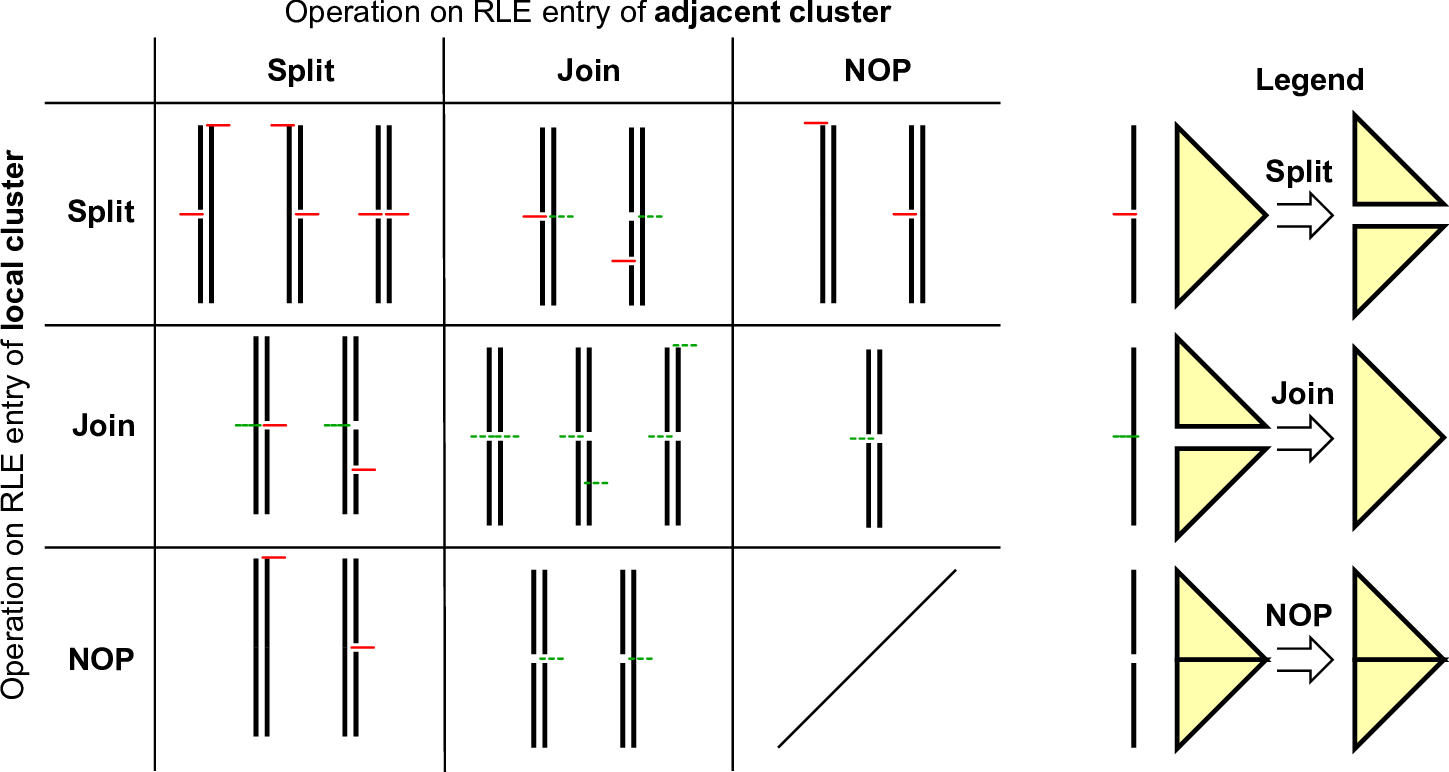
Given the rules introduced in the previous algorithm, we discuss the relevant scenarios given in left image in Fig. 5.15 for cluster b by traversing the adjacent clusters.
Left image:
Right image:
Algorithm: Local RLE entry update - adjacent transfer state: JOINED_CHILD
In case of a joined adjacent child, the local RLE is tested for the possibility to join it with the next local RLE. Such a join is producing a consistent state in case that both consecutively stored adjacently joined children have the same parent. Otherwise, this would result in a violation of our assumption of a unique RLE existing for shared interfaces, see Sec. 5.2.3. Other updates of the RLE meta information can be applied similarly to the split case above.
Algorithm: Local RLE entry update - adjacent transfer state: NO_TRANSFER
With all local RLE entries being updated directly in case of split and join operations, no modifications of the RLE entry are required in case of an adjacent cluster without split/join.
Algorithm: Postprocessing RLE updates
Finally, the possibly RLE meta information which was duplicated to avoiding race conditions (see step 4 in the ’outer loop’ part of the algorithm above) is used as the new RLE meta information.
This algorithm computes a consistent meta information fulfilling all theorems described so far in this thesis.
We like to give a short outlook to distributed-memory parallelization: Here, we use two-sided communication and the read-only push/pull principle: We separate the updates of the meta information into local and adjacent operations. Instead of looking up the required split/join information by accessing the adjacent clusters stored at another MPI node, our updates of the meta information for each local RLE entry rely on a cooperative communication:
All local clusters send the necessary split/join information about their local changes to the adjacent clusters (push). The adjacent clusters can then receive (pull) this data and update the meta communication information similar to the shared memory synchronization. This leads to a straightforward extension of the shared-memory algorithm presented above.
We have not considered the vertex communication meta information for dynamic clustering, yet. After cluster splits and joins, the vertex communication meta information can be in an inconsistent state since zero-length encoded vertex RLE entries can be missing. However, we can reconstruct the vertex communication information based on a valid edge communication from the previous section.
The algorithmic idea is based on the assumption that all clusters sharing the vertex also store one or two edge-related RLE meta information about edge-adjacent clusters (or a boundary) which also share the vertex. By accessing the edge-adjacent clusters, we can continue our search to the other vertex-sharing clusters. Then all clusters sharing a vertex can be traversed via following the RLE edge communication information associated to this vertex. This allows generation of a trace of all clusters sharing the vertex and, based on this trace, a reconstruction of our zero-length encoded vertex RLE meta information.
Without loss of generality, we only show the algorithm with the assumption that both SFC traversal directions along the hyperfaces shared by two clusters are in opposite directions.
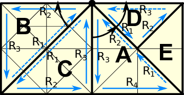
For each cluster Pi, let the left and right RLE edge communication meta information be given by Rk({left,right}) = (Q,m)k with Q the adjacent cluster, m > 0 the number of edges shared with the adjacent partition and 1 < k < N({left,right}) selecting the RLE entry. The cluster associated to the first entry in the tuple Rj = (Q,m) is given by P(Rj) := Rj[1] == Q.
We use a flag F ∈{front,back} describing whether the vertex for which the meta information is determined is associated to the front or back of the currently processed edge-related RLE entry. For the sake of convenience, we formally2 combine R({left,right}) to a single ring-like buffer of RLE meta information

Algorithm: Reconstruction of vertex meta information for cluster Pi
For all Rj ∈ R of the cluster Pi, execute the following operations:
In case that P(current) represents a boundary, we set the flag F to front and continue the search with P(current) := P(Rj+1). If this is also a boundary, the vertex is not shared by any other cluster and we stop the algorithm.
(I) In case that this is the second time that we run into a boundary, we visited all adjacent clusters which are connected via edges and the algorithm terminates.
(II) Otherwise, we rerun our trace generation (1) on the start cluster P(prev) := Pi but traversing in the other direction P(current) := P(Rj+1). The flag F is then set to front.
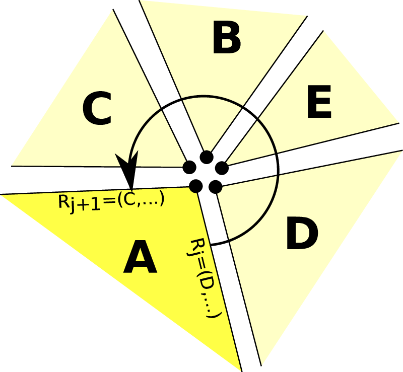
Based on the visited clusters, we can reconstruct the required RLE vertex meta information. For each RLE, at most 8 adjacent clusters which share the vertex are visited. Therefore, this algorithm has a constant runtime for each RLE. Furthermore, the algorithm is based on local (only vertex-adjacent) access operations only. Giving the average number of RLE elements per cluster in avgRLE, the runtime complexity is O(#Cluster ⋅ avgRLE).
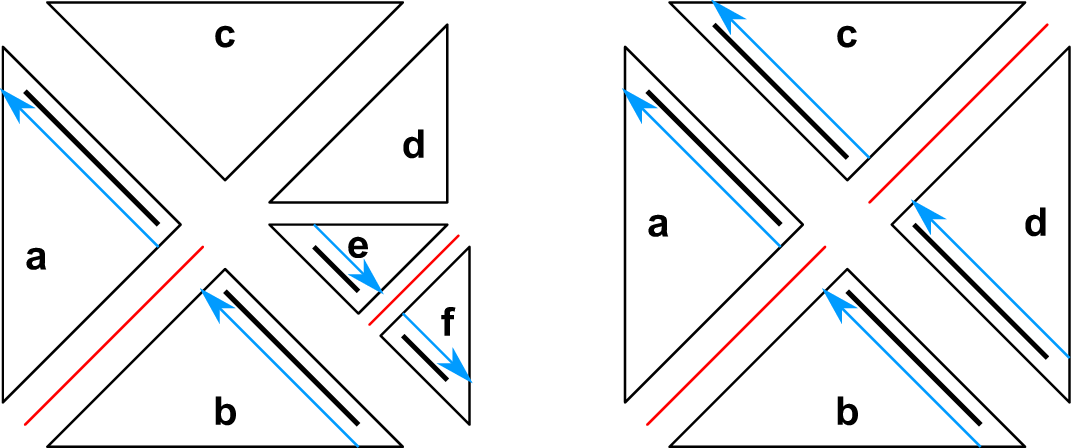
We give a concrete example of this algorithm for reconstructing the RLE information for cluster C and the middle vertex at the top in Fig. 5.17. Here, we start with the RLE entry R3 := (A,.) and initialize the algorithm to P(prev) := C, P(current) := A and F := back.
Due to the detected boundary, we set F := front, P(prev) := C and P(current) := Rj+1 = B.
We also like to mention an alternative way which was not implemented in this work: The information on the adjacently generated vertices can also be inferred similar to the reconstruction of edge meta information, see Sec. 5.5.3. With this method, we can also search on the adjacent split/joined cluster meta information for a possible requirement of inserting or removing vertex RLE meta information.