
Discretizing the time step term from Eq. (2.9). We can factor out U by considering that φ are functions only depending on spatial parameters. This yields
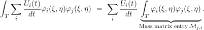 | (2.10) |
The integrals on the right-hand side of Eq. (2.10) can then be precomputed and their values stored to
the mass matrix . Using vector notation  , we get a matrix-vector formulation
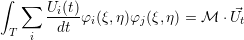 | (2.11) |
with  also a matrix in case of several conserved quantities.
See Appendix A.1 for examples of matrices derived in this section and used in our simulations. Those matrices are computed with Maple1 , a computer algebra system for symbolic computations.
Applying the explicit Euler time-stepping method, this can then be rearranged to
