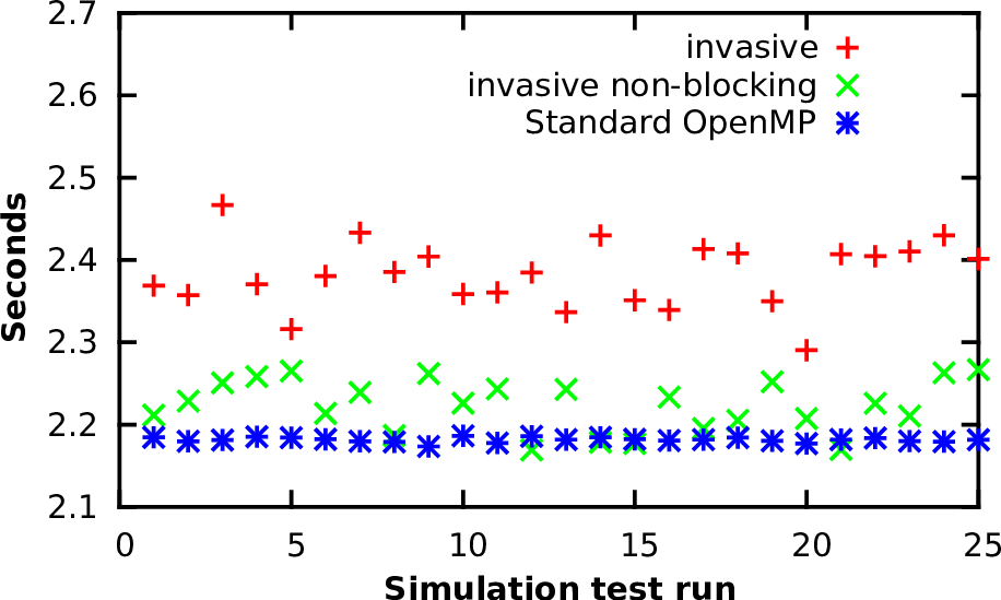
Figure 8.3: Plot of the seconds taken for each of 25 simulation runs and for each application
type: non-invasive with OpenMP, invasive with blocking communication to the RM and invasive
with non-blocking communication.
This section presents several studies in the context of our formerly described Invasive Computing implementation for HPC shared-memory systems.
We start with overhead measurements of our Invasive Computing interfaces comparing the blocking with the non-blocking (re)invade calls. For a measurement in a realistic environment, we use the simulation framework presented in the previous part and start several small shallow water simulations on a grid which is regularly refined with 128 cells. The invasive versions are realized with extensions to OpenMP.
We analyzed the invasive overheads with three different versions:
The invasive versions of the simulations send one invade request to the resource manager between each time step. The measurements of the overall application’s runtime were conducted for 25 executions of a single application. It is sufficient to consider a single application, since we are currently only interested in the overheads of the RM. The required simulation times on a single core are printed in Fig. 8.3. The blocking version of the invasion leads to an overhead of 15% in average compared to the non-invasive version. However, this invasion is compensated by the non-blocking version, yielding a robust improvement compared to the blocking one and results in an overhead of only 5% in average compared to the non-invasive version. Hence, we continue running our invasive benchmarks with the non-blocking version.
Our main motivation for Invasive Computing in the area of HPC was driven by simulations on dynamically adaptive grids. Next, we use our shallow water simulation to show the functionality of dynamic resource distribution based on scalability graphs.
The scalability graphs we use are determined in advance with the execution of simulations for a few time steps on different cores and different refinement parameters. An example of such scalability graphs with different grid cells is given in Fig. 8.4, it was computed on the platform Intel, a 40-core shared-memory system (see Appendix A.2). Given a particular number of grid cells, e.g. based on the current number of cells used in the dynamically adaptive simulation, the scalability graph can be extracted by a slice.
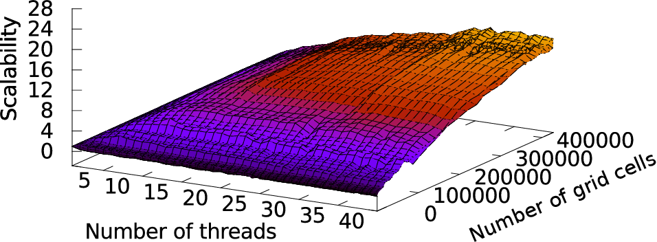
We can then optimize the resource distribution with the precomputed scalability graphs: Given the number of current grid cells, we determine the scalability graph which is closest to the given number of grid cells. Such a scalability graph is one slice of the plot in Fig. 8.4. If the scalability graph is different to the previous one, it is forwarded to the RM. We can then run multiple shallow water simulations in parallel without oversubscribed resources and the resources optimized by the RM with the scalability graph.
For the benchmark scenario, we use four identical shallow water simulations. Each one is started slightly delayed to the previous one with 10, 20, and 10 seconds. The simulation mesh is initialized with an initial refinement depth of 4 and 14 additional adaptivity levels. The splitting threshold is set to 8192.
Based on the scalability graphs, the dynamic resource redistribution of concurrently executed applications which are started shortly delayed is presented in Fig. 8.5. The resource distribution is based on the scalability optimization algorithm presented in Section 8.4.
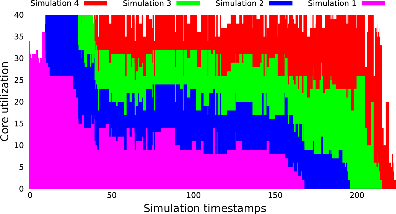
Having a closer look on the execution times, the invasive version took 266 seconds for its execution. We compare this execution time with an OpenMP parallelization which executes the simulations one after another. This resulted in an execution time of 521 seconds. Our approach is also competitive to a TBB parallelized version which starts the simulation as soon as it is enqueued, taking 491 seconds for the execution. Here, the Invasive Computing shows a clear benefit with an improvement of 49% compared to the OpenMP parallelization and 46% if comparing it to the TBB parallelized execution.
To show the real potential of Invasive Computing in the context of an application with an iterative time-stepping scheme, we use a scenario of several Tsunami parameter studies in parallel. Here, we use the Tohoku Tsunami simulation which was presented in Sec. 6.3. Here, the simulation first loads the bathymetry datasets, then preprocesses it to a multi-resolution format and initializes the simulation grid. Finally, the wave propagation is simulated.
As a parameter study, we executed five simulations with slightly different adaptivity parameters. Since starting all simulations at the same time does not yield a realistic HPC scheduling, the enqueuing of the executions of each of these simulations is delayed with the seconds given in the following vector: (10,15,15,15).
We challenge OpenMP and TBB with our Invasive Computing approach, yielding three different parallelization methods:
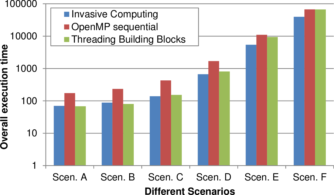
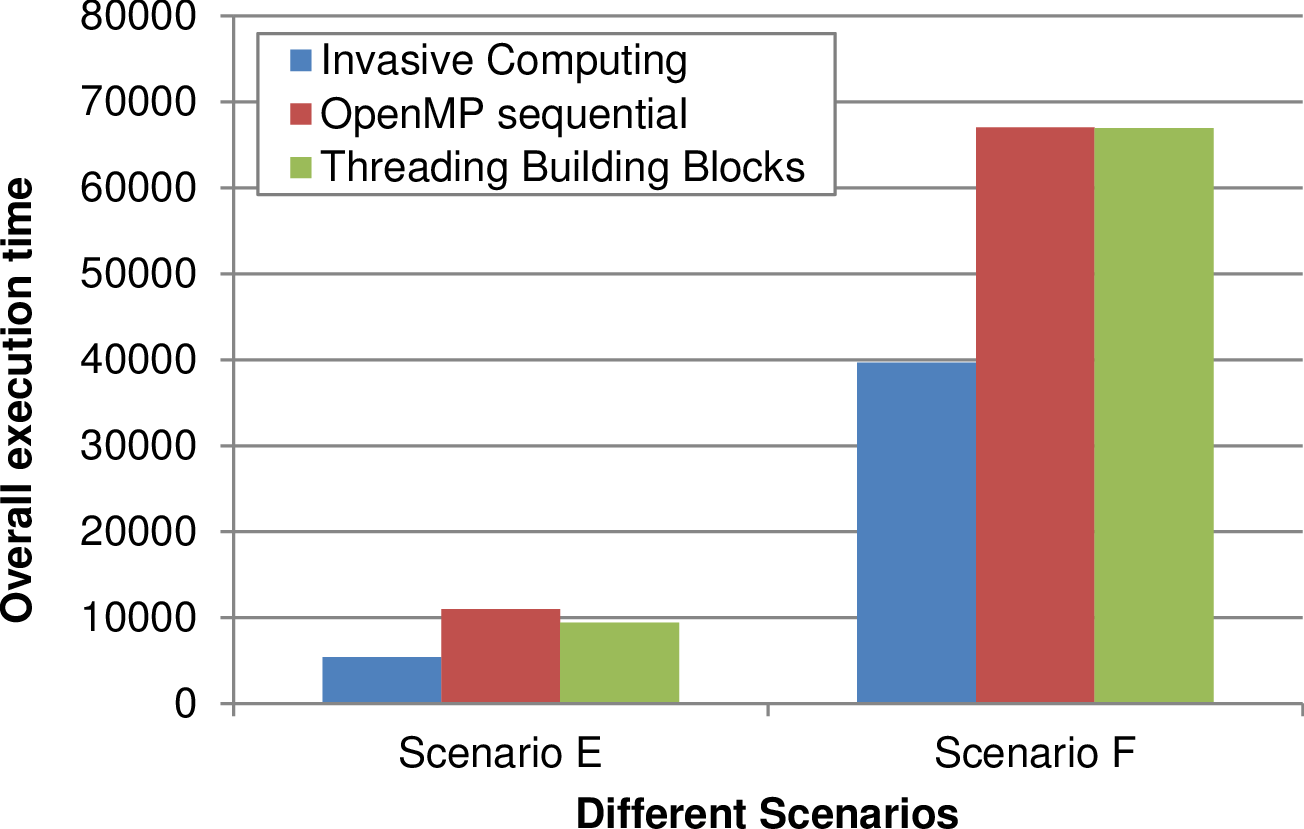
The overall execution time for several scenarios, each one based on five simulations, is depicted in Fig. 8.6 for different problem sizes. These problem sizes of the simulations in each scenario are increased from left to right by increasing the initial refinement depth. The adaptivity refinement depth of (10,10,8,8,7) was used for the five simulations.
For smaller problem sizes, TBB yielded optimizations similar to our Invasive Computing approach. However, these problem sizes were only considered for testing purpose and do not yield any practical relevant data. For larger simulations as they were considered for the analysis of our Tsunami simulations in Section 6.3, TBB looses its performance improvement compared to the OpenMP non-invasive execution.
We further depicted the results of the scenarios E and F with a larger problem size and a linear scaling in the right image in Fig. 8.6. Here, our Invasive Computing approach leads to a robust performance improvement of 45% compared to a non-invasive parallelization with standard OpenMP and TBB.
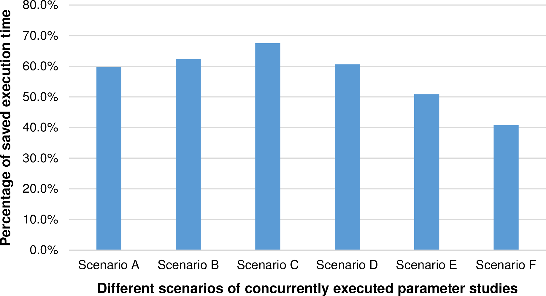
Assuming a simulation executed with a sufficiently large workload, a close-to-linear scalability can be reached, see Sec. 5.7. Since the performance improvements of Invasive Computing rely on a non-linear scalability of applications and furthermore a scalability which is changing over the runtime, we further analyzed the behavior of the performance improvements of the invasive execution from small to large simulation scenarios. We plotted the reduction in runtime in percentage comparing the invasive to the non-invasive execution in Fig. 8.7. Here, we can see that the performance improvements with Invasive Computing are less for larger simulation scenarios. We account for that by the improved scalability of larger workloads.
We close this chapter by relating our results to a concrete example for the da = 22∕0 Tsunami simulation from Sec. 6.3. This simulation has an overall execution time of 2557.11 seconds and we assume, that the execution time of scenarios E has the closest similarity regarding the runtime. Then, assuming concurrently executed parameter studies of this workload, the improvement in efficiency is above 50%.