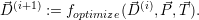
 is computed based on the previously introduced
data structures
is computed based on the previously introduced
data structures  as the specified optimization target and
  as an per-application specified
information.
as an per-application specified
information.
The content and structure of this section is related to our work [SRNB13b] which is currently under
review. The optimized target resource distribution is computed based on the previously introduced
data structures as the specified optimization target and as an per-application specified
information.
We further drop the core dependencies of our original optimization function (8.2), yielding the simplified optimization function
 | (8.3) |
Optimizations are then applied with the constraints of all applications depending on  and the
per-application optimization target
and the
per-application optimization target  .
.
Requirements on constraints: The constraints which are forwarded by resource-aware applications
to the RM are then kept in  with one entry for each application. Then, the RM schedules the
available resources based on the optimization target and these constraints. Here, we distinguish
between local (optimizing resources for a single application) and global constraints (optimizing
resources for multiple applications).
with one entry for each application. Then, the RM schedules the
available resources based on the optimization target and these constraints. Here, we distinguish
between local (optimizing resources for a single application) and global constraints (optimizing
resources for multiple applications).
Local constraints: With constraints given by the range of cores between 1 and the maximum number of cores, an application can request a particular range of cores. These constraints make is challenging to optimize concurrently running applications since no knowledge on their performance state for a changing number of resources can be inferred and we refer to such constraints as local ones.
Global constraints: Such constraints can be evaluated by the optimization function in a way which optimizes the resources targeting at a global optimum of all applications.
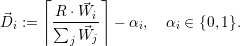
 i resources to the application
  i. To avoid over-subscription (see
Eq. (8.1)), α has to be chosen in a particular way.
i. To avoid over-subscription (see
Eq. (8.1)), α has to be chosen in a particular way.
With the assigned number of resources  i, the problem can be reformulated to a scalability
optimization. Here, we assume that each application has a perfect strong scalability S(c)
for c cores within the range [1;
i, the problem can be reformulated to a scalability
optimization. Here, we assume that each application has a perfect strong scalability S(c)
for c cores within the range [1; i] and no performance gain beyond
  i cores:
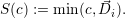
For a given number of cores c, the throughput T(c) represents the fraction of time to
compute a solution for a fixed problem size w =  i. Next, we consider the throughput
improvement for a changing number of cores with the baseline given at the throughput
of a single core:
i. Next, we consider the throughput
improvement for a changing number of cores with the baseline given at the throughput
of a single core:  =
=  =: S(c). This yields the relation to the scalability graph of
strong scalability S(c). Hence, we can use the scalability graph as an optimization hint
for the application’s throughput. Furthermore, we can use a scalability graph to optimize
for the theoretical global maximum throughput even among heterogeneous applications
due to the normalization S(1) = 1 for a single core.
=: S(c). This yields the relation to the scalability graph of
strong scalability S(c). Hence, we can use the scalability graph as an optimization hint
for the application’s throughput. Furthermore, we can use a scalability graph to optimize
for the theoretical global maximum throughput even among heterogeneous applications
due to the normalization S(1) = 1 for a single core.
Let the scalability graph Si(c) be provided by application  i. We further require a strictly
monotonously increasing behavior
i. We further require a strictly
monotonously increasing behavior

The global throughput is then maximized by searching the most efficient resource-to-application
combination in  . This yields a multi-variate maximization problem in
  j for our optimization
target
j for our optimization
target
 | (8.4) |
Again, we avoid over-subscription with the side constraint ∑
j j ≤ R.
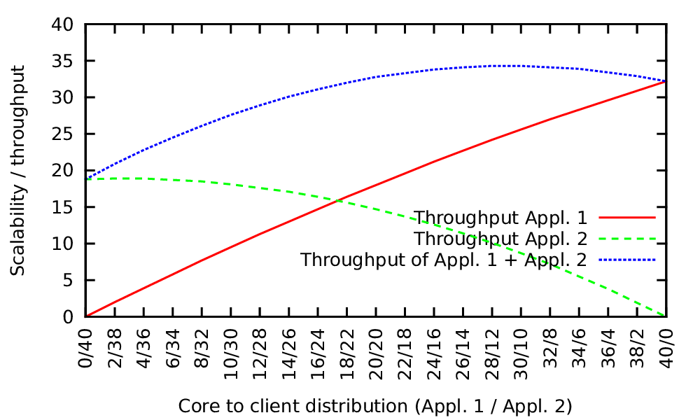
Fig. 8.2 shows an example of such an optimization. Two applications are considered which provide a scalability graph. The graph with the red solid line represents the scalability of the first application with increasing number of resources from left to right and the green dashed line represents the scalability graph of the second application with the numbers of resources increasing from right to left.
To optimize the resource distribution for our “maximizing throughput” optimization target, the optimal point is given by the maximum of the sum of both throughput graphs.
However, we can use our requested properties of strictly monotonously increasing and concave scalability graphs. This allows us to solve the maximization problem for an arbitrary number of applications with an iterative gradient method which is related to the steepest descent solver [FP63] and assuming that there is only one optimum, the global optimum.
Initialization: The iteration vector  (k) for the k-th iteration is introduced which assigns
  i
computing cores to each application i. We start with
i
computing cores to each application i. We start with  (0) := (1,1,…,1) which assigns each
application a single core at the start. This is required since each application demands for at least
a single core on which it is executed.
(0) := (1,1,…,1) which assigns each
application a single core at the start. This is required since each application demands for at least
a single core on which it is executed.
Iteration: We then compute the throughput improvement for each application i, for a single core additionally assigned to it:
 | (8.5) |
Then, the application n, which yields the maximum throughput improvement is given by ΔSn := maxj{ΔSj}.
We can update the resource distribution for the k + 1-th iteration by
 | (8.6) |
with the Kronecker symbol δ.
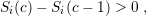
Stopping criterion: If all resources are distributed (∑
i i(k) = R), we can stop our optimization
and the last iteration vector
i(k) = R), we can stop our optimization
and the last iteration vector  contains the optimized target resource distribution for
 (k+1).