5.7 Results: Shared-memory parallelization

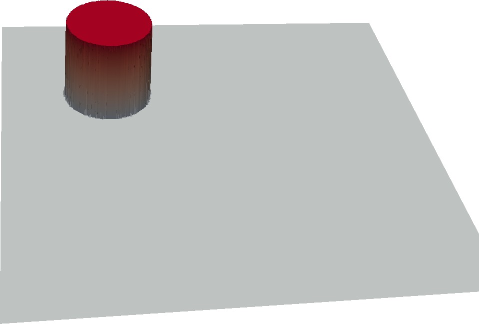
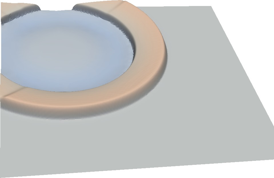
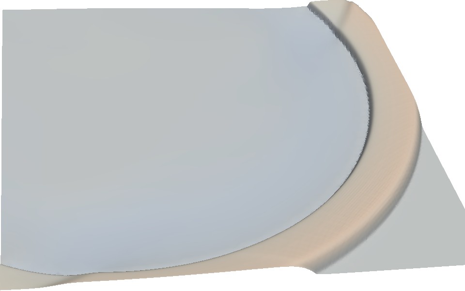
Figure 5.21: Visualization of three different time steps for a representative radial dam break test scenario. A radial dam break is used for most of the benchmarks in this section [SWB13a].

We conducted several benchmarks with the test platforms further denoted as Intel and AMD. All computations are done in single precision. A sketch of a shallow water benchmark which is simulating a radial dam break is given in Fig. 5.21. Detailed information on both systems is given in Appendix A.2.

The first benchmark scenario is given by a flat sea-ground 300 meters below the sea surface and a domain length of 5 km. We use up to 8 levels of refinements and allow the refinement/coarsening triggered according to the surface above/below 300.02/300.01 meter. Our domain is set up by two triangles forming a square centered at the origin. The initial refinement depth is given by d, resulting in 2^d+1 coarse triangles without adaptivity. The dam is placed with its center at (-1250m,1000m) with a radius of 250m. The positive water displacement is set to 1m. Performance results are given in “Million Cells Per Second” (MCPS) that can be computed.

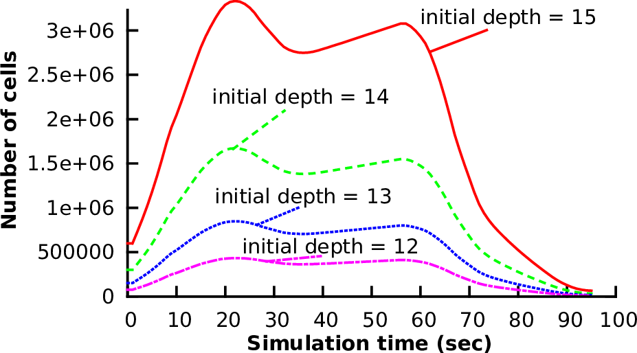
The dynamically changing number of cells over the entire simulation is given in Fig. 5.22. A visualization of a similar scenario with an initial radial dam break is given in Fig. 5.21.

Threshold-based split size

With the threshold-based cluster generation approach (see Sec. 5.6.2), we expect overheads introduced depending on the number of clusters (i.e. on the maximum number of cells in each cluster). The following benchmark is based on a regular and non-adaptive grid. We tested different initial refinement depths d, each depth resulting in a grid with 2^d+1 cells. The simulation is based on 1^st-order spatial- and time-discretization of the shallow water equations.

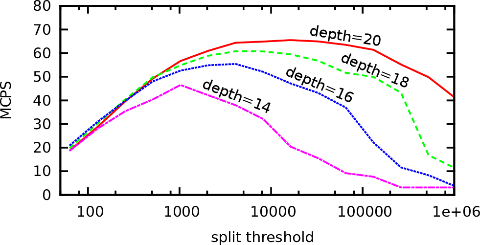
The results in Fig. 5.23 show the dependency of the efficiency on the cluster split threshold. We account for these performance increases and decreases with tasking overheads, synchronization requirements and load imbalances. These aspects are further described and performance increase and decrease is depicted with ↑ and ↓, respectively, in the following table:

Thus, the optimal performance depends on the problem size, the number of cores and the splitting of the clusters.

Threading overhead

We continue with a more detailed analysis of the overheads introduced by threading and, if not otherwise mentioned, fix the split threshold size to T_s := 32768, i.e. the number of clusters is kept constant. Several benchmark settings were used:

• Serial: This version is based on the serial software design, see Fig. 4.12. In particular, no cluster set is used and no threading overheads exist.
• Parallel, no splitting, 1 thread: This version and the upcoming described versions are based on the parallel software design, see Fig. 5.10. The splitting threshold was set to infinity.
• Parallel, 1 thread: The simulation was executed with a single thread and the cluster generation is based on the cluster split threshold size T_s.
• Parallel, N threads: The simulation was executed with N threads in parallel with the cluster split threshold size T_s.

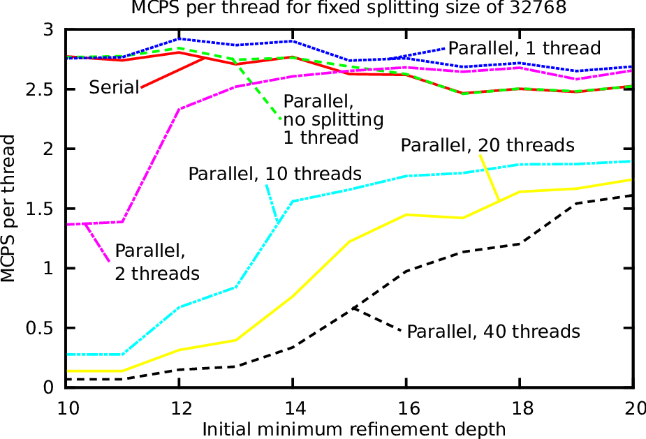
The threads are pinned to non-hyperthreaded cores in a compact way. A simulation domain set up by a single base triangle with a typical radial dam break scenario was used. The maximum refinement depth was set to 8 and 100 simulated seconds were computed. The results, based on the million processed cells per second divided by the number of threads, are given in Fig. 5.24. The benchmarks were conducted on the platform Intel and we discuss the benchmark data in the order of the test runs.

• Serial: The serial version slows down after a refinement depth of 12 to 14. The reason for this is the problem size exceeding a cache level size.
• Parallel, no splitting, 1 thread: This version almost coincides with the serial version. Thus, we can conclude that almost no overhead is introduced by the additional layers for the parallelization.
• Parallel, 1 thread: With a larger problem size, we see that a parallel approach leads to an improved performance compared to the serial version only. Detailed traversal statistics show a performance improvement in both the simulation and adaptivity traversals.

  We account for this improved performance with a cache-blocking effect: Our clustering splits the domain into independent chunks with a size of equal or less than 2¹⁵ = 32768. This generates clusters with a size also fitting at least into the last-level cache. To account for the temporal data reaccesses which is required for such a cache effect, we reconsider our stack access strategies between traversals:

  (a) In the edge-based communication scheme used in this implementation, we pushed the flux DoF stored on both edges to a buffer and computed the fluxes after the cluster’s grid was traversed. Thus, the DoF stored on this buffer can still be available in cache and accessed with less latency.

  (b) Regarding the adaptivity traversals, we only use the structure and adaptivity stack as input. In our implementation, we only access 2 bytes on the structure and 1 byte for the adaptivity state stack for each traversed cell during the traversals generating a conforming grid. This perfectly fits into a higher cache level. By atomically executing the forward traversal directly after a backward traversal in one operation executed on the cluster, the structure and adaptivity information is still kept in a higher cache level and thus does not have to be written back to main memory.

• Parallel, N threads: The simulation was executed with N threads in parallel. Effects based on the cache-optimizations of the single-threaded version above could also be measured for the 2-threaded simulation.

  For higher number of threads (10, 20 and 40), no further improvements due to cache-blocking could be gained for the considered problem sizes. Simulations and the scalability with a larger number of threads are discussed in the next sections.

We conclude that our approach leads to optimizations with cache-aware cluster sizes and, hence, can lead to a memory bandwidth reduction for dynamically adaptive meshes.

Strong-scaling benchmarks

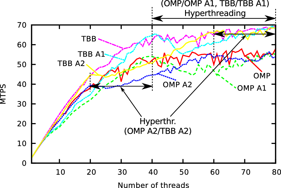
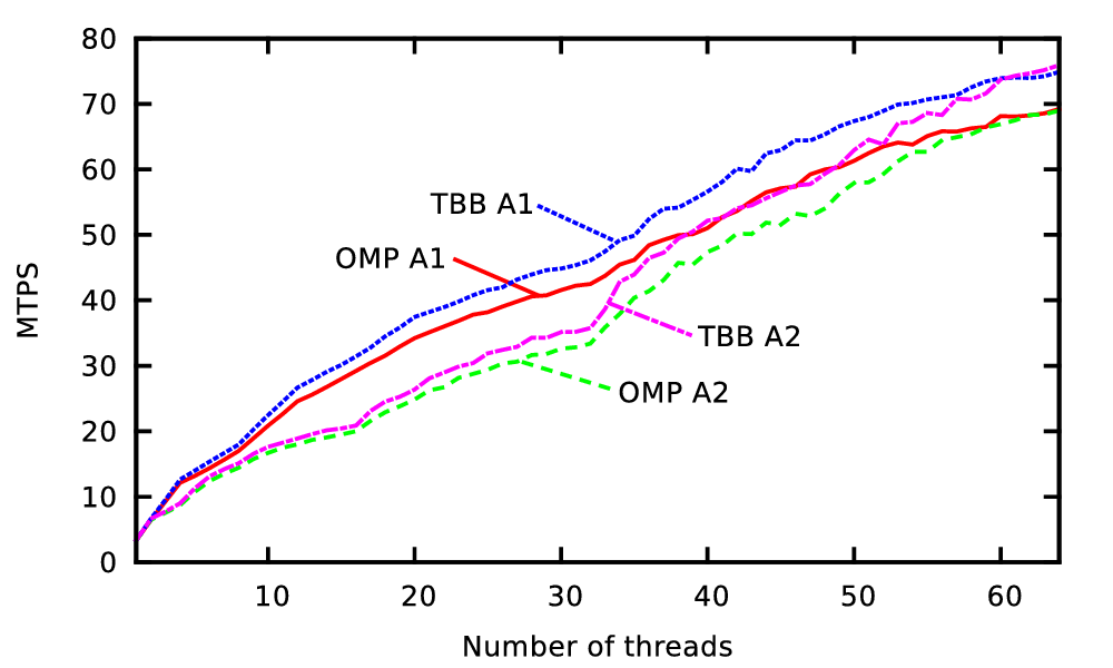
We continue with strong-scaling benchmarks on shared-memory test platforms Intel and AMD (see Appendix A.2). On the Intel platform, the first 40 cores are the physical ones, followed by 40 cores which are the hyperthreaded ones. The simulations were initialized with a minimum refinement depth of 20. During the setup of the radial dam break, we use up to 8 additional refinement levels. We computed 100 time steps, leading to about 19 Mio. grid cells processed in average per time step. Tasking from TBB and OpenMP was used for the evaluation.

If not stated differently, we consider NUMA domain effects and try to avoid preemptive scheduling with context switches by pinning threads to computing cores. This is also referred as setting the thread affinities. We evaluated three different core-affinity strategies:

• no affinities: This implementation does not use any pinnings. Thus, the threads can be preemted and their execution continues on another core.
• A1: This pins all threads in a linearly increasing manner following the core enumeration. On platform Intel, the enumeration is priorized first with all non-hyperthreaded cores on a socket, then over all sockets, followed by all hyperthreaded cores on all sockets. The first 10 threads are then pinned to the non-hyperthreaded cores on the first socket, the next 10 threads to the second socket, etc. Threads 41 to 50 are pinned to the hyperthreaded cores.
• A2: Assuming a core enumeration starting with 1, this pinning skips every second core until all odd-numbered cores are consecutively assigned. The next threads are then pinned to the even-numbered cores. With our platform Intel and using 40 threads with A2 affinities, this results in the first 20 threads being assigned to the odd-numbered physical cores followed by the odd-numbered hyperthreaded cores on all sockets.

The results for the platform Intel and AMD are given in Fig. 5.25 and 5.26 and are discussed next.

• Platform Intel:
  Using TBB, the best scalability can be measured for this platform with A1 scheduling. With the A2 scheduling, the scalability gets worse after 20 threads due to threads 21 to 40 being assigned to the hyperthreaded cores with their non-hyperthreaded cores already used for computations.

  With OpenMP, less scalability is gained in general for the considered test case. We created tasks with the untied clause for each cluster tree node. Due to known issues for OpenMP task constructs (see e.g.  [OP09]), the scalability is not as good for unbalanced trees as by using TBB for parallelization.

• Platform AMD:
  Sufficient scalability could be also determined for the AMD platform with an overall performance close to the Intel system. Since the considered AMD platform shares the floating point units (FPU) for 2 particular cores in the architecture, we account for the bend visible at multiples of 8 for A1 and A2 affinities by this FPU sharing.

Strategies for scheduling and cluster generation

We next consider different combinations for scheduling, determining which thread executes computations on which clusters (see Sec. 5.6.1) and how to dynamically generate clusters (see Sec 5.5). The benchmark scenario is based on a 2^nd-order discretization in space and 1^st-order discretization in time.

Regarding the scheduling stragtegies, we shortly recapitulate them in the following table:

We also developed two different cluster-generation approaches shortly recapitulated in the next table:

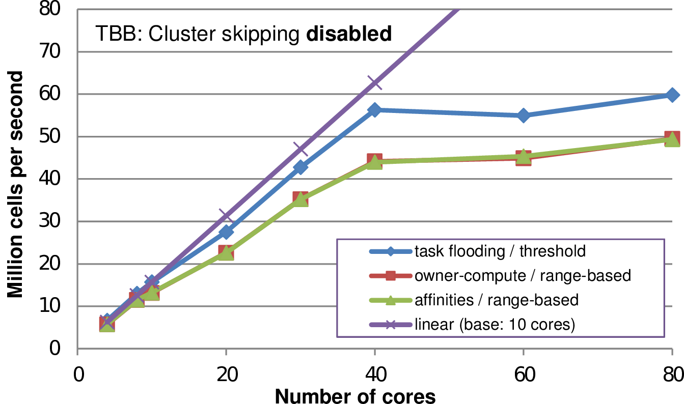
We conducted benchmarks with different combinations of the above mentioned scheduling and cluster generation strategies (See Fig. 5.27). Here we see that a cluster generation approach with range-based treesplits does not result in improvements as expected, but leads to less performance. We account for that by additional splits and joins compared to the pure threshold-based method. Such splits and joins of clusters result in additional overhead due to synchronizing updated meta information and additional memory access to split and join the cluster. Using a threshold-based cluster generation, by far less changes due to cluster splits and joins are required. This leads to improved performance for the threshold-based clustering.